Rep:LMD:jjb215

Overview: Well written report, I like your intro and you've completed all the tasks. Just the heat cap, hopefully my comment clears it up! In terms of style, you use "this does this" and "this means that" a bit too much - for your thesis this/next year, ensure you use synonyms and spiced up language or it becomes a bit monotonous! Mark 68/100

Abstract

Not bad just be careful that your conclusions aren't too general

The dynamical properties of a Lennard-Jones system was investigated using molecular dynamics simulations. The variation of density with temperature and pressure, along with the variation of the heat capacity with the density and temperature were examined. The radial distribution functions of the solid, liquid and gas phases were used to describe the structures of each of these phases-- showing that the solid phase has a long range, ordered lattice structure, whereas the liquid and gas phases have no long range order and contain atoms that are very diffuse. Does a liquid have no long-range order? Diffusion coefficients were calculated for all three phases using the mean squared displacement (MSD) and velocity autocorrelation function (VACF): solid phase with -2.57 x 10^-6 m²s^-1 (MSD) and 2.02 x 10^-5 m²s^-1 (VACF); liquid phase with 0.0860 m²s^-1 (MSD) and 0.0783 m²s^-1 (VACF); the gas phase with 2.08 m²s^-1 (MSD) and 2.14 m²s^-1 (VACF). An idea could be to compare the VACF + msd methods to measure the diffusion coefficient and make a comment on your conclusions here

Introduction

Good, I like how you've tried to tailor the work to an audience. I know it's a bit time-constrained but would be good here to have some sort of literature overview too.

Phase changes occur in everyday life, such as the boiling of water using a kettle, rain which falls under gravity due to the condensation of atmospheric water vapour (precipitation) and the evaporation of perfume from the skin. More specifically, most perfumes are manipulated to have a three-part smell, which are released at different times after application. The top notes are released within the first 15 minutes of application on the skin, heart notes emerge after around 3-4 hours and finally, the base notes are the last to evaporate-- which appear after around 6 hours. The release of these smells is governed by phase changes-- liquid to gas. The controlled release of fragrances is an interesting area of research and more specifically, the incorporation of perfumes in polymers for the purpose of prolonged delivery (at a constant rate) over a period of 12 or more hours. Research into phase changes can open new doors to the way fragrances are produced-- they can be fine-tuned to have a more controlled release of each of the three notes and can be personalised to the oiliness or the dryness of the skin.

The use of molecular dynamics (MD) simulations allows investigation of a system of particles and subsequent extraction of thermodynamic properties such as the system's total energy, temperature, pressure and density. MD simulations provide a quick and easy way of investigating a particular system under controlled conditions without needing to physically set up an experiment. Modelling systems using the Lennard-Jones (L-J) potential allows computation of heat capacity, diffusion coefficient and even the structure of the system through the use of radial distribution functions (RDF). Measurement of heat capacities and diffusion coefficients is of large interest in the perfumery industry as being able to understand and control these physical properties allows for a much finer control in the way perfume evaporates or stay on the skin.

Aims and Objectives

• Investigating the dependence of computational accuracy on timestep
  • Finding the appropriate timestep to use in simulations
• Investigating the density of the system as a function of pressure and temperature
• Examining the heat capacity as a function of temperature
• Examining the change in structure of the system using RDFs
• Finding the diffusion coefficient of the solid, liquid and gas phase using two methods:
  • Mean squared displacement
  • Velocity autocorrelation function

Methods

Good, I like how you've started describing the model and moved onto tools as we discussed.

All the simulations were run using a Lennard-Jones potential and were run using LAMMPS.

Figure 1: Structure of the simple cubic (sc) lattice

Figure 2: Structure of the face-centered cubic (fcc) lattice

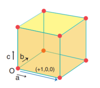
The model used in these simulations is a simple cubic (sc) lattice with a number density of 0.8 to give a lattice spacing in x, y, z = 1.07722, 1.07722, 1.07722-- where atoms are placed on each of the lattice points. A simulation box size of 15 x 15 x 15 lattice spacings is created and the box contains only a single species of atom. The mass of the atoms created is set to 1.0, the pairwise interactions are computed using the L-J potential with a cutoff distance of 3.0 (in reduced units). The pairwise L-J force field coefficients are also set to 1.0 for the potential well depth ($ϵ$) and 1.0 for the zero-potential distance ($\sigma$). The atoms were then assigned random velocities, whilst ensuring that the Maxwell-Boltzmann distribution was still followed by the system.

The above model was used in equation of state simulations using an NpT ensemble and specifying the desired temperature and pressure of the system. Twenty-two phase points were chosen by varying the temperature (T* = 2.0, 2.5, 3.0, 3.5, 4.0, 4.5, 5.0, 5.5, 6.0, 8.0, 10.0) and pressure (P* = 1.8, 2.6).

Heat capacity simulations were run at ten phase points-- $\rho *$ = 0.2, 0.8 and $T*$ = 2.0, 2.2, 2.4, 2.6, 2.8. The system was brought to the desired state in the NVT ensemble and once the system was in the correct thermodynamic state, the thermostat is turned off and the NVE ensemble is used.

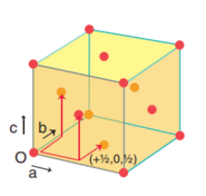
Calculations of the radial distribution functions (RDF) were done by specifying the correct number density and temperature to give the desired phase. For the solid phase (uses the fcc lattice), $N$ = 1.2, $T*$ = 1.0; for the liquid phase, $N$ = 0.8, $T*$ = 1.2 and for the gas, $N$ = 0.08, $T*$ = 1.2. The L-J cutoff has also been changed from 3.0 to 3.2.

In the simulations to calculate the mean squared displacement (MSD) and velocity autocorrelation function (VACF), the densites and temperatures used to give the desired phase are the same to the ones used in RDF simulations. The L-J cutoff used is still 3.2; however, the size of the simulation box has been changed to 20 x 20 x 20.

The following relationships were used to calculate the diffusion coefficients: $D=\frac{1}{6}\frac{\partial ⟨r^2\left(t\right)⟩}{\partial t}$ for the MSD method and $D=\frac{1}{3}\underset{0}{\overset{\mathrm{\infty }}{\int }}\mathrm{d}\tau ⟨\mathbf{v}\left(0\right)\cdot \mathbf{v}\left(\tau \right)⟩$ for the VACF method.

Results and Discussion

Equation of state

Figure 3: Average density against average temperature of the system, along with the ideal gas law.

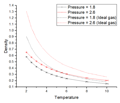
From figure 3, it can be seen that the density predicted by the ideal gas law is higher than the densities obtained from the simulations. This is because the ideal gas law assumes point particles and perfect elastic collisions are the only iteractions they experience-- this causes the density to be higher as it ignores the short order repulsive interactions. On the contrary, the L-J systems contain short order repulsive terms which causes the particles of the system to be further apart; hence, the densities arising from the simulations are lower than what is predicted by the ideal gas law. Tick

At higher pressures, the discrepancy increases because the number density increases with pressure and this causes a decrease in the cell volume. This means that the particles are closer together and there is an increase in collisions and in the repulsive interactions of the system. This increase in repulsion means that the system behaves further away from ideality. However, this discrepancy decreases and the L-J system behaves closer to ideality as the temperature is increased. This can be explained as being due to the system having enough energy to escape and not be isolated in the L-J potential well-- the system has more freedom to move along its potential energy surface and this makes the simulated L-J system behave more like an ideal gas. You're overusing "this" - "this... this... this..." - be careful, try to get some synonyms.

It can also be seen that as the temperature is increased, the number density decreases and this is because the atoms have more kinetic energy and therefore, the average distance between atoms increases. And as the number density decreases, the closer the L-J system is to ideality and this is because the system experiences less repulsive interactions.

Heat capacity

Figure 4: C_v/V against temperature

The heat capacity is a measure of how easily the temperature of a substance can be increased-- it is a measure of the amount of energy required to increase the temperature. From figure 4, it can be seen that the heat capacity of the substance decreases as the temperature is increased. This is because as the temperature increases, the particles occupy more states in the higher excited energy levels (ie. higher density of states in the higher energy levels) and at higher energy levels, the energy gap between the levels decrease. This decrease in the energy gap means that it becomes increasingly easier to populate higher energy levels; thus, causing the heat capacity to decrease with temperature. There's a bit of a misunderstanding here - between the inherent chemical properties of a system and what changing these properties would mean for the heat capacity and simulating the heat capacity over our simulation of Lennard-Jones particles. In our simulation, and what I've tried to get people previously to suggest, we see a slight decrease in heat capacity with increasing temperature. What do we expect? Constant number of particles.. Internal enegy remains constant.. Cv = dU/dT and thus constant heat capacity. If I changed the material or the particles and changed the DOS or inherent properties of the systme, the heat capacity would vary as you suggest.

The heat capacity is also seen to increase with density because there are more atoms per unit volume and therefore, more states per unit volume-- higher density of states. This means don't overuse "this means" that more states have to be populated in order to raise the temperature of the system. This leads to the substance requiring more energy in order to excite all the atoms in the more dense system, which causes the increase in the heat capacity.

Radial distribution function

Figure 5: RDF as a function of r for different phases

Figure 6: Integral of RDF as a function of r for different phases

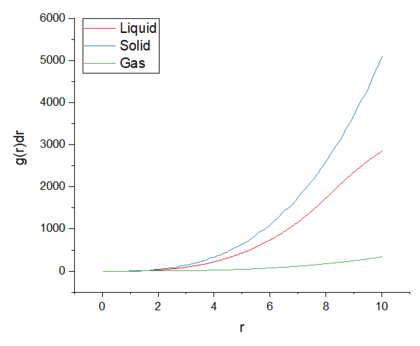From the RDFs shown in figure 5, the position of the coordination spheres are indicated by the peaks and the empty space (where there are no atoms) between these spheres is indicated by the troughs. In the solid phase, the peaks are sharper due to the regular crystal lattice, where the atoms have a fixed position but still under go some vibrational motion. Due to the short range and long range order of the coordination spheres, the peaks are sharper compared to other phases. The slow decay to the bulk density value is also due to the short and long range order of the crystal lattice. The first three peaks of the solid phase RDF shows the first three coordination spheres around the central reference atom. Using the integral of the RDF in figure 6, the number of atoms in these coordination spheres can be found.

Table 1: Coordination number of the first three peaks in the solid phase

Distance from reference atom, r	g(r)dr	Co-ordination Number
1.275	12.01315	12
1.625	17.97563	6
1.975	42.26231	24

Figure 7: The first, second and third nearest neighbours in the solid phase

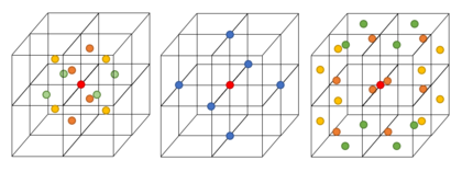
The lattice spacing is calculated from $\rho =\frac{N}{V}$, where $\rho =1.2$ and $N=4$ (due to fcc lattice)-- the lattice spacing is 1.494. The coordination numbers for the first three peaks in the solid phase RDF are 12, 6 and 24, respectively.

The liquid phase RDF contains less and broader peaks-- this is due to the lower order structure and the atoms not being held tightly in position. The first peak at around r = 1 indicates the first coordination shell and the small peaks indicate the short range structure of the liquid. The RDF however decays quickly to the bulk density value due to the atoms being able to move, becoming more diffuse as r increases and therefore, the liquid loses its structure at long distances. The RDF of the gas phase shows one broad peak and then very quickly decays to the bulk density value. This is because gases do not have a regular structure nor a long range order. This means that there is only a single coordination shell and at further distances away from the central reference atom, the atoms are very diffuse. Tick, g(r) does indeed give us info into the long-range order of a system

Diffusion coefficient using MSD and VACF

MSD method:

Nice graphs!

Figure 8: Solid phase MSD against time for own simulation

Figure 9: Liquid phase MSD against time for own simulation

Figure 10: Gas phase MSD against time for own simulation

Figure 11: Solid phase MSD against time for 1, 000, 000 atoms

Figure 12: Liquid phase MSD against time for 1, 000, 000 atoms

Figure 13: Gas phase MSD against time for 1, 000, 000 atoms

Table 2: Diffusion coefficients using the MSD method

Phase	Diffusion coefficient m2s-1
	Default simulation	1, 000, 000 atoms simulation
Solid	-2.57 x 10-6	-8.43 x 10-6
Liquid	0.0860	0.0873
Gas	2.08	3.02

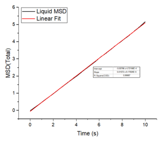
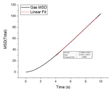
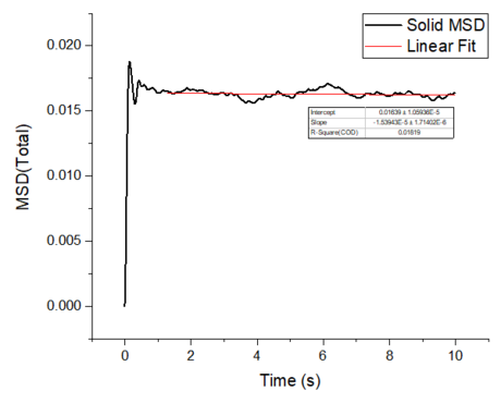
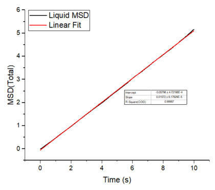
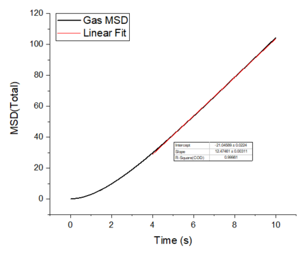
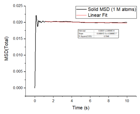
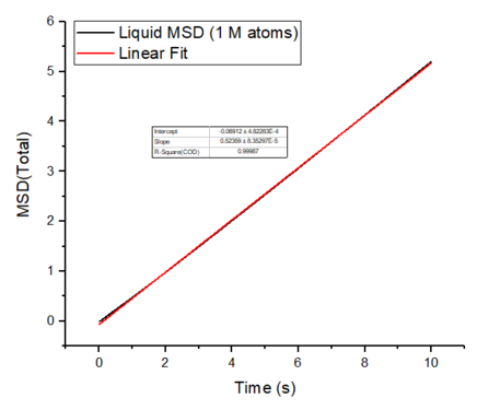
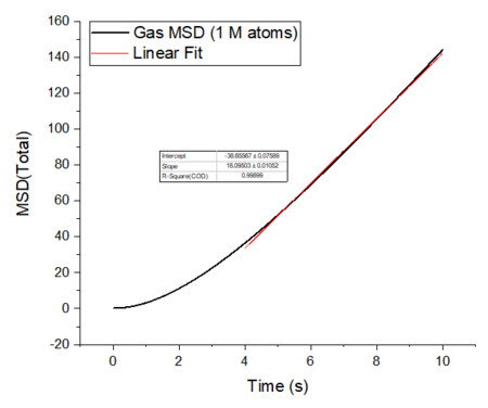
The mean squared displacement plots behave as expected for each phase. The solid phase MSD shows that the atoms have a fixed position in the lattice; however, the atoms are still able to vibrate but not able to diffuse away from their regular lattice structure. This is seen from the small oscillating behaviour of the MSD-- showing that the atoms stay roughly at their position over time. In the case of liquid and gas phases, the MSD increases over time and this indicates that the atoms of the system are able to diffuse away from the reference position.

In the diffusive region, the MSD and time have a linear relationship ($$\begin{gathered} MSD \\ \alpha \\ {t}^x \end{gathered}$$, where $x=1$). Good knowledge of the power law The diffusion coefficients have been calculated using the gradients of the MSD plots in the diffusive region for each of the phases and these are shown in table 2. The gas phase has the highest diffusion coefficient as the atoms are very disperse and experience minimum interactions-- this is supported by its RDF, where it was shown that the atoms in the gas phase are very diffuse and have a very low order structure. The liquid phase has a lower diffusion coefficient due to the initial short range order and weak attractive interactions the atoms experience to hold the structure together. The solid phase has the lowest diffusion coefficient and this is because it has a highly ordered crystal lattice structure, where the atoms are not able to translate far away from their fixed position but instead, they only experience vibrational motion. The initial large spike in the MSD is due to the ballistic region, where the system has not yet reached equilibrium and the MSD does not change linearly with time.

The diffusion coefficients obtained from the default simulations compare closely to the simulations containing one million atoms. The diffusion coefficients obtained from the larger systems are more accurate because of the larger amount data that contributes to the average MSD. Tick

VACF method:

Figure 14: VACFs of solid, liquid and harmonic oscillator

Figure 15: VACF integral against time for default simulation

Figure 16: VACF integral against time for 1, 000, 000 atoms

Table 3: Diffusion coefficients using the VACF method

Phase	Diffusion coefficient m2s-1
	Default simulation	1, 000, 000 atoms simulation
Solid	2.02 x 10-5	4.55 x 10-5
Liquid	0.0783	0.0901
Gas	2.14	3.27

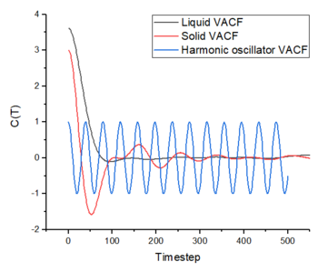
In figure 15, the minima and maxima of the solid and liquid VACF correspond to the forwards and backwards motion of the atoms, where their velocites are reversed after each oscillation. In other words, the atoms change their direction of motion after each collision. However, the magnitude of these oscillations dampen due to the interactions experienced by the atoms-- disrupting the oscillatory motion (the velocity decorrelates over time). The difference in the solid and liquid VACFs is that the oscillatory motion of the liquid decays more quickly due to the higher diffusion coefficient of the liquid phase and the atoms become much more dispersed compared to the solid phase. This higher diffusion coeffcient also causes the liquid VACF to have fewer initial oscillations, due to the fewer initial collisions between atoms. The larger number of oscillations in the solid VACF is due to more initial collisions, which is caused by the regular close packing of the lattice. The first and only minimum in the liquid VACF can be considered as the point where all the atoms have collided at least once before they rebound from each other and diffuse away. tick

The harmonic oscillator VACF differs from both phases in that the oscillation does not decay over time. The harmonic oscillator assumes the atoms of the system do not lose energy-- which explains the undecaying oscillatory motion. It does not include the long range attractive and short range repuslive interactions experienced by the L-J system-- which causes the dampening on the solid and liquid VACFs.

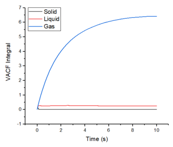
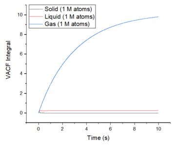
The diffusion coeffcients have been calculated using the integrals of the VACFs and these were calculated using the trapezoidal rule. The values obtained are as expected for each of the phases and they also compare closely to the values obtained from using the MSD method. The values obtained from the default simulations are also very close to the ones obtained from the larger systems. However, the largest source of error in the estimates of the diffusion coefficients comes from using the trapezoidal rule to approximate the integral. At a maximum, the integral is underestimated and at a minimum, the integral is overestimated. Good

Conclusion

The equation of state was examined by running simulations of multiple phase points (by varying the temperature and pressure) and it was found that increasing the temperature decreased the density, whilst increasing the pressure caused an increase in the density. The deviation of the L-J system compared to the ideal gas law is found to be due to the fact that L-J potential includes short range repulsive interactions that causes a decrease in the number density.

The dependence of heat capacity with temperature was investigated and it was found that the heat capacity decreased due to the decreasing energy gap at higher energy states. And with increasing density, it was found that the heat capacity increased and this was due to an increase in the density of states that need to be populated in order to increase the temperature. Evaluation of heat capacities is essential to creating new fragrant molecules in perfumes, as it is one of the important properties that control the release of the perfume from the skin.

The RDFs were used to describe the structure of each of the phases. The RDFs showed that the structure of the solid phase has a long range order and that the liquid and gas phases showed little to no long range order, respectively. The quick decay of the liquid and gas RDFs to the bulk density value is due to the atoms being able to diffuse far away from the reference atom-- causing the loss of oscillations in the RDF. The large number of oscillations and the slow decay of the solid phase RDF reveals the regular and rigid long range order of the lattice-- the atoms are not able to diffuse far away from the reference atom and therefore, are able to form many coordination shells.

Diffusion coefficients for all three phases were calculated using the MSD and VACF. The values obtained were as expected: the solid phase has a very low diffusion coefficient of -2.57 x 10^-6 m²s^-1 (MSD) and 2.02 x 10^-5 m²s^-1 (VACF); liquid phase with 0.0860 m²s^-1 (MSD) and 0.0783 m²s^-1 (VACF); the gas phase with 2.08 m²s^-1 (MSD) and 2.14 m²s^-1 (VACF). As with heat capacity, examining the diffusion coefficients of substances and new molecules paves the way into designing better perfumes, in terms of being able to have a better control of their release.

Tasks

These are nicely done! Tick

Section One

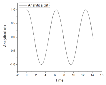
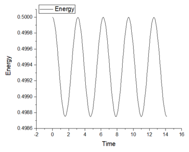
1. Open the file HO.xls. In it, the velocity-Verlet algorithm is used to model the behaviour of a classical harmonic oscillator. Complete the three columns "ANALYTICAL", "ERROR", and "ENERGY": "ANALYTICAL" should contain the value of the classical solution for the position at time $t$, "ERROR" should contain the absolute difference between "ANALYTICAL" and the velocity-Verlet solution (i.e. ERROR should always be positive -- make sure you leave the half step rows blank!), and "ENERGY" should contain the total energy of the oscillator for the velocity-Verlet solution. Remember that the position of a classical harmonic oscillator is given by $x\left(t\right)=A\cos (\omega t+\varphi )$ (the values of $A$, $\omega$, and $\varphi$ are worked out for you in the sheet).

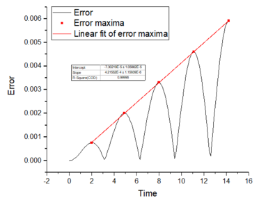
2. For the default timestep value, 0.1, estimate the positions of the maxima in the ERROR column as a function of time. Make a plot showing these values as a function of time, and fit an appropriate function to the data.

Figure 1: Analytical x(t) for the harmonic oscillator

Figure 2: Total energy of the harmonic oscillator

Figure 3: Error between analytical and velocity-Verlet algorithm

HO excel file for the two tasks above

3. Experiment with different values of the timestep. What sort of a timestep do you need to use to ensure that the total energy does not change by more than 1% over the course of your "simulation"? Why do you think it is important to monitor the total energy of a physical system when modelling its behaviour numerically?

A low timestep of at least 0.2 is required as the highest total energy change is 1% over the course of the simulation. It is important to monitor the total energy in computational work because the calculation methods used (Velocity-Verlet algorithm) use approximations and there will be fluctuations in the values obtained (total energy). Monitoring and decreasing these fluctuations is important in accurately modelling the realistic behaviour of a physical system. From this task, it is clear that decreasing the timestep will decrease the energy fluctuations and provide more accurate results; however, this causes an increase in the length of the simulation. Finding the right balance between simulation time and accuracy is key to many computational experiments.

HO excel file for varying timestep

4. For a single Lennard-Jones interaction, $\varphi \left(r\right)=4ϵ(\frac{{\sigma }^{12}}{r^{12}}-\frac{{\sigma }^6}{r^6})$, find the separation, $r_0$, at which the potential energy is zero. What is the force at this separation? Find the equilibrium separation, $r_{eq}$, and work out the well depth ($\varphi \left(r_{eq}\right)$). Evaluate the integrals $\underset{2\sigma }{\overset{\mathrm{\infty }}{\int }}\varphi \left(r\right)\mathrm{d}r$, $\underset{2.5\sigma }{\overset{\mathrm{\infty }}{\int }}\varphi \left(r\right)\mathrm{d}r$, and $\underset{3\sigma }{\overset{\mathrm{\infty }}{\int }}\varphi \left(r\right)\mathrm{d}r$ when $\sigma =ϵ=1.0$.

Separation $r_0$:

$\varphi \left(r_0\right)=4ϵ(\frac{{\sigma }^{12}}{r_0^{12}}-\frac{{\sigma }^6}{r_0^6})=0$

$\frac{{\sigma }^{12}}{r_0^{12}}-\frac{{\sigma }^6}{r_0^6}=0$

$\frac{{\sigma }^{12}}{r_0^{12}}=\frac{{\sigma }^6}{r_0^6}$

$\frac{{\sigma }^{12}}{{\sigma }^6}=\frac{r_0^{12}}{r_0^6}$

${\sigma }^6=r_0^6$

$r_0=\sigma$

Force at $r_0$:

$F(r)=-\frac{d\varphi (r)}{dr}$

$=4ϵ(\frac{12{\sigma }^{12}}{r_0^{13}}-\frac{6{\sigma }^6}{r_0^7})$

$=24ϵ(\frac{2{\sigma }^{12}}{r_0^{13}}-\frac{{\sigma }^6}{r_0^7})$

$r_0=\sigma$:

$F=24ϵ(\frac{2{\sigma }^{12}}{{\sigma }^{13}}-\frac{{\sigma }^6}{{\sigma }^7})$

$=24ϵ(\frac{2}{\sigma }-\frac{1}{\sigma })$

$=\frac{24ϵ}{\sigma }$

Equilibrium separation, $r_{eq}$:

$\frac{d\varphi (r)}{dr}=4ϵ(-\frac{12{\sigma }^{12}}{r^{13}}+\frac{6{\sigma }^6}{r^7})=0$

$12\frac{{\sigma }^{12}}{r^{13}}=6\frac{{\sigma }^6}{r^7}$

$2{\sigma }^6=r^6$

$r_{eq}=2^{1/6}\sigma$

Potential well depth:

$\varphi (r)=4ϵ(\frac{{\sigma }^{12}}{(2^{1/6}\sigma {)}^{12}}-\frac{{\sigma }^6}{(2^{1/6}\sigma {)}^6})$

$=4ϵ(\frac{{\sigma }^{12}}{4{\sigma }^{12}}-\frac{{\sigma }^6}{2{\sigma }^6})$

$=4ϵ(\frac{1}{4}-\frac{1}{2})$

$=-ϵ$

Integrals when $\sigma =ϵ=1.0$:

$\int \varphi \left(r\right)\mathrm{d}r=\int 4(\frac{1}{r^{12}}-\frac{1}{r^6})dr=4(-\frac{1}{11r^{11}}+\frac{1}{5r^5})$

$\underset{2\sigma }{\overset{\mathrm{\infty }}{\int }}\varphi \left(r\right)\mathrm{d}r=-0.0248$

$\underset{2.5\sigma }{\overset{\mathrm{\infty }}{\int }}\varphi \left(r\right)\mathrm{d}r=-8.18\times 10^{-3}$

$\underset{3\sigma }{\overset{\mathrm{\infty }}{\int }}\varphi \left(r\right)\mathrm{d}r=-3.29\times 10^{-3}$

5. Estimate the number of water molecules in 1ml of water under standard conditions. Estimate the volume of $10000$ water molecules under standard conditions.

Assumption that 1 mL of water is 1 g, the number of molecules of water is N_A/18 = 3.35 x 10²² molecules. 10, 000 molecules of water is 10, 000/N_A = 1.66 x 10^-20 moles. The mass in g is then 1.66 x 10^-20 x 18 = 2.99 x 10^-19 g, and because 1 mL is approximately 1 g, the volume is 2.99 x 10^-19 mL.

6. Consider an atom at position $(0.5,0.5,0.5)$ in a cubic simulation box which runs from $(0,0,0)$ to $(1,1,1)$. In a single timestep, it moves along the vector $(0.7,0.6,0.2)$. At what point does it end up, after the periodic boundary conditions have been applied?

$(0.5,0.5,0.5)+(0.7,0.6,0.2)=(0.2,0.1,0.7)$ (due to periodic boundary conditions

The Lennard-Jones parameters for argon are $$\begin{gathered} \sigma =0.34\mathrm{n}\mathrm{m},ϵ \\ / \\ {k}_B=120\mathrm{K} \end{gathered}$$. If the LJ cutoff is $r^{*}=3.2$, what is it in real units? What is the well depth in $$\begin{gathered} {\mathrm{k}\mathrm{J} \\ \mathrm{m}\mathrm{o}\mathrm{l}}^{-1} \end{gathered}$$? What is the reduced temperature $T^{*}=1.5$ in real units?

LJ cutoffː

$r^{*}=\frac{r}{\sigma }=3.2$

$r=3.2\times 0.34$

$$\begin{gathered} =1.088 \\ nm \end{gathered}$$

Well depth:

$ϵ=120k_B{N}_A\times 10^{-3}$

$$\begin{gathered} =0.998 \\ kJmo{l}^{-1} \end{gathered}$$

Temperature:

$T*=\frac{T}{120}$

$T=120\times 1.5$

$$\begin{gathered} =180 \\ K \end{gathered}$$

Section Two

Why do you think giving atoms random starting coordinates causes problems in simulations? Hint: what happens if two atoms happen to be generated close together?

If atoms are generated too close to each other, then they can experience a strong repulsive interaction and thus, these atoms would have very large potential energies. This could make it difficult for the system being modelled reach equilibrium due to the large total energy of the system.

Satisfy yourself that this lattice spacing corresponds to a number density of lattice points of $0.8$. Consider instead a face-centred cubic lattice with a lattice point number density of 1.2. What is the side length of the cubic unit cell?

$\rho =\frac{N}{V}$

$=\frac{1}{1.07722^3}=0.8$

For FCC

$V=L^3=\frac{4}{1.2}$

$L=\sqrt[3]{\frac{4}{1.2}}=1.494$

Consider again the face-centred cubic lattice from the previous task. How many atoms would be created by the create_atoms command if you had defined that lattice instead?

A FCC lattice contains four atoms and in a 10x10x10 simulation box, there would be 4000 atoms.

Using the LAMMPS manual, find the purpose of the following commands in the input script:

mass 1 1.0
pair_style lj/cut 3.0
pair_coeff * * 1.0 1.0

'mass 1 1.0' sets the mass of atom type 1 as 1.0

'pair_style lj/cut 3.0' sets the formulas LAMMPS uses to compute pairwise interactions. Lennard-Jones potential is chosen and with a cutoff distance of 3.0-- where pair potentials are defined between pairs of atoms that are within this cutoff distance of 3.0.

'pair_coeff * * 1.0 1.0' sets the pairwise force field coefficients for one or more pairs of atom types. The coefficients for the Lennard-Jones potential are the well depth and the distance at zero potential.

Given that we are specifying ${\mathbf{x}}_i\left(0\right)$ and ${\mathbf{v}}_i\left(0\right)$, which integration algorithm are we going to use?

The Velocity-Verlet algorithm

Look at the lines below.

### SPECIFY TIMESTEP ###
variable timestep equal 0.001
variable n_steps equal floor(100/${timestep})
timestep ${timestep}

### RUN SIMULATION ###
run ${n_steps}
run 100000

The second line (starting "variable timestep...") tells LAMMPS that if it encounters the text ${timestep} on a subsequent line, it should replace it by the value given. In this case, the value ${timestep} is always replaced by 0.001. In light of this, what do you think the purpose of these lines is? Why not just write:

timestep 0.001
run 100000

By using a global variable, it is easy to modify the input files as only a single value needs to be changed-- the value where the variable was initialised. The values of the 'timestep' and 'n_steps' will be changed in the whole script.

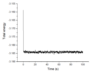
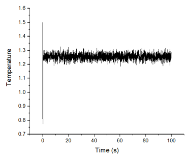
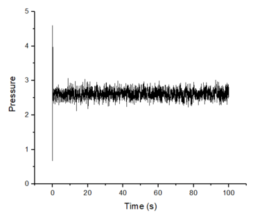
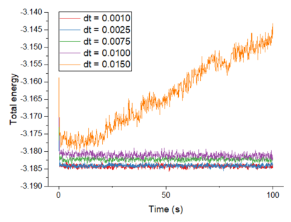
Make plots of the energy, temperature, and pressure, against time for the 0.001 timestep experiment (attach a picture to your report). Does the simulation reach equilibrium? How long does this take? When you have done this, make a single plot which shows the energy versus time for all of the timesteps (again, attach a picture to your report). Choosing a timestep is a balancing act: the shorter the timestep, the more accurately the results of your simulation will reflect the physical reality; short timesteps, however, mean that the same number of simulation steps cover a shorter amount of actual time, and this is very unhelpful if the process you want to study requires observation over a long time. Of the five timesteps that you used, which is the largest to give acceptable results? Which one of the five is a particularly bad choice? Why?

Figure 4: Plot of total energy against time for 0.001 timestep

Figure 5: Plot of temperature against time for 0.001 timestep

Figure 6: Plot of pressure against time for 0.001 timestep

Figure 7: Plot of total energy against time for varying timesteps

The simulation using 0.0010 timestep reaches equilibrium in about 0.2 s. Of the five timesteps, 0.0025 is the largest timestep that gives acceptable results as it gives around the same convergence value as the 0.0010 timestep. This allows more actual time to be covered over a certain number of simulation steps. This is more practical when simulating over longer periods of time and the calculation time would be lower for a certain length of simulation without losing accuracy. The worst choice of timestep is 0.0150 because the system does not reach equilibrium and instead, the system's total energy increases.

Choose 5 temperatures (above the critical temperature $T^{*}=1.5$), and two pressures (you can get a good idea of what a reasonable pressure is in Lennard-Jones units by looking at the average pressure of your simulations from the last section). This gives ten phase points — five temperatures at each pressure. Create 10 copies of npt.in, and modify each to run a simulation at one of your chosen $(p,T)$ points. You should be able to use the results of the previous section to choose a timestep. Submit these ten jobs to the HPC portal. While you wait for them to finish, you should read the next section.

We need to choose $\gamma$ so that the temperature is correct $T=\mathfrak{𝔗}$ if we multiply every velocity $\gamma$. We can write two equations:

$\frac{1}{2}\sum _i{m}_i{v}_i^2=\frac{3}{2}N{k}_{B}T$

$\frac{1}{2}\sum _i{m}_i{\left(\gamma v_i\right)}^2=\frac{3}{2}N{k}_B\mathfrak{𝔗}$

Solve these to determine $\gamma$.

$\frac{\frac{1}{2}\sum _i{m}_i{\left(\gamma v_i\right)}^2}{\frac{1}{2}\sum _i{m}_i{v}_i^2}=\frac{\frac{3}{2}N{k}_B\mathfrak{𝔗}}{\frac{3}{2}N{k}_{B}T}$

${\gamma }^2=\frac{\mathfrak{𝔗}}{T}$

$\gamma =\sqrt{\frac{\mathfrak{𝔗}}{T}}$

Use the manual page to find out the importance of the three numbers 100 1000 100000. How often will values of the temperature, etc., be sampled for the average? How many measurements contribute to the average? Looking to the following line, how much time will you simulate?

The three values are assigned to Nevery, Nrepeat and Nfreq, respectively. Nevery specifies the interval at which input values are sampled for the average (every 100 timesteps in this case). Nrepeat specifies the number of input values that are used for the average (1000 sets of input values). Nfreq specifies at what timestep the average is calculated (timestep 100000 in this case). This means over the 100, 000 simulation steps, 1000 samples of the data contribute to the average and the data is sampled every 100 timestep. Since, the timestep used is 0.00250 and there are 100, 000 timesteps, then the amount of time simulated is 250 s.

When your simulations have finished, download the log files as before. At the end of the log file, LAMMPS will output the values and errors for the pressure, temperature, and density $\left(\frac{N}{V}\right)$. Use software of your choice to plot the density as a function of temperature for both of the pressures that you simulated. Your graph(s) should include error bars in both the x and y directions. You should also include a line corresponding to the density predicted by the ideal gas law at that pressure. Is your simulated density lower or higher? Justify this. Does the discrepancy increase or decrease with pressure?

Figure 8: Average density against average temperature of the system, along with the ideal gas law.

The density predicted by the ideal gas law is higher than the densities obtained from the simulations. This is because the ideal gas law assumes point particles and perfect elastic collisions are the only interactions they experience-- this causes the density to be much higher. The L-J system contains short range repulsive interactions and hence, the particles in the simulated system are further apart compared to the ideal gas system-- causing the simulated densities to be lower than ideal.

At higher pressures, the discrepancy increases as the number density increases due to a decrease in the volume-- this forces the particles to be closer together and have increased repulsive interactions. This increase in repulsive forces between particles in the simulation causes a larger deviation from ideality. At higher temperatures, the discrepancy decreases due to the system having enough kinetic energy to move away and not be localised in the L-J potential well-- the system has more freedom moving along its potential energy surface and this makes the simulated system behave more like an ideal gas.

Section Three

As in the last section, you need to run simulations at ten phase points. In this section, we will be in density-temperature $({\rho }^{*},T^{*})$ phase space, rather than pressure-temperature phase space. The two densities required at $0.2$ and $0.8$, and the temperature range is $2.0,2.2,2.4,2.6,2.8$. Plot $C_V/V$ as a function of temperature, where $V$ is the volume of the simulation cell, for both of your densities (on the same graph). Is the trend the one you would expect? Attach an example of one of your input scripts to your report.

Figure 9: C_v/V against temperature

The heat capacity of the system decreases with increasing temperature. This is expected because as the temperature increases, the particles have a higher density of states in the excited state and at higher excited states, the energy gap between the levels decreases -- it becomes increasingly easier to populate higher energy levels. This causes the heat capacity to decrease with temperature. The heat capacity also increases with density because the system contains more energy levels that need to be populated in order to increase the temperature of the system.

Example of input file

Section Four

Perform simulations of the Lennard-Jones system in the three phases. When each is complete, download the trajectory and calculate $g(r)$ and $\int g(r)\mathrm{d}r$. Plot the RDFs for the three systems on the same axes, and attach a copy to your report. Discuss qualitatively the differences between the three RDFs, and what this tells you about the structure of the system in each phase. In the solid case, illustrate which lattice sites the first three peaks correspond to. What is the lattice spacing? What is the coordination number for each of the first three peaks?

Figure 10: RDF as a function of r for different phases

Figure 11: Integral of RDF as a function of r for different phases

The RDF for the gas phase shows one broad peak and quickly decays to g(r) = 1. This is becauuse Be careful to read through for typos! gases do not have a regular structure and do not have a long range order. This means that the gas phase only has a single coordination shell and at a further distance r, the atoms are very diffuse and hence decay to the bulk density value. The RDF of the liquid phase contains three broad peaks and slowly decays to the bulk density value. The decay is due to the atoms being able to move, becoming more diffuse as r increases and therefore, the liquid loses its structure at long distances. The peaks indicate the initial short range structure and the coordination shells of the liquid phase. The solid phase RDF contains a large number of peaks and decays very slowly compared to other phases. This is because the solid phase has a long range and regular structure-- where the atoms have fixed positions. The peaks correspond to the many coordination shells of the reference particle, including the long range structure of the lattice. Tick

Figure 12: The first, second and third nearest neighbours in the solid phase

The lattice spacing is calculated from $\rho =\frac{N}{V}$, where $\rho =1.2$ and $N=4$ (due to fcc lattice)-- the lattice spacing is 1.494. The coordination numbers for the first three peaks in the solid phase RDF are 12, 6 and 24, respectively.

Section Five

Make a plot for each of your simulations (solid, liquid, and gas), showing the mean squared displacement (the "total" MSD) as a function of timestep. Are these as you would expect? Estimate $D$ in each case. Be careful with the units! Repeat this procedure for the MSD data that you were given from the one million atom simulations.

Figure 13: Solid phase MSD against time for own simulation

Figure 14: Liquid phase MSD against time for own simulation

Figure 15: Gas phase MSD against time for own simulation

Figure 16: Solid phase MSD against time for 1, 000, 000 atoms

Figure 17: Liquid phase MSD against time for 1, 000, 000 atoms

Figure 18: Gas phase MSD against time for 1, 000, 000 atoms

Table 1: Diffusion coefficients using the MSD method

Phase	Diffusion coefficient m2s-1
	Default simulation	1, 000, 000 atoms simulation
Solid	-2.57 x 10-6	-8.43 x 10-6
Liquid	0.0860	0.0873
Gas	2.08	3.02

The mean squared displacement plots behave as expected for each phase. The solid phase MSD shows that the atoms have a fixed position in the lattice; however, the atoms are still able to vibrate but not able to diffuse away from their regular lattice structure. This is seen from the small oscillating behaviour of the MSD-- showing that the atoms stay roughly at their position over time. In the case of liquid and gas phases, the MSD increases as the time increases and this indicates that the atoms of the system are able to diffuse away from their positions. The gas phase has the highest diffusion coefficient (slope) as the atoms are very disperse and experience minimum interactions. The linear region is due to the diffusive regime-- where the atoms move further away from the reference position over time.

In the theoretical section at the beginning, the equation for the evolution of the position of a 1D harmonic oscillator as a function of time was given. Using this, evaluate the normalised velocity autocorrelation function for a 1D harmonic oscillator (it is analytic!):

$C\left(\tau \right)=\frac{\underset{-\mathrm{\infty }}{\overset{\mathrm{\infty }}{\int }}v\left(t\right)v(t+\tau )\mathrm{d}t}{\underset{-\mathrm{\infty }}{\overset{\mathrm{\infty }}{\int }}{v}^2\left(t\right)\mathrm{d}t}$

Be sure to show your working in your writeup.

Differentiation of the 1D harmonic oscillator ($x\left(t\right)=A\cos (\omega t+\varphi )$)

$\frac{\partial x}{\partial t}=v\left(t\right)=-\omega A\sin (\omega t+\varphi )$

$C\left(\tau \right)=\frac{\underset{-\mathrm{\infty }}{\overset{\mathrm{\infty }}{\int }}{\omega }^2{A}^2\sin (\omega t+\varphi )\sin (\omega (t+\tau )+\varphi )\mathrm{d}t}{\underset{-\mathrm{\infty }}{\overset{\mathrm{\infty }}{\int }}(-\omega A\sin (\omega t+\varphi ){)}^2\mathrm{d}t}$

Expanding and then cancelling:

$C\left(\tau \right)=\frac{\underset{-\mathrm{\infty }}{\overset{\mathrm{\infty }}{\int }}\sin (\omega t+\varphi )\sin (\omega (t+\tau )+\varphi )\mathrm{d}t}{\underset{-\mathrm{\infty }}{\overset{\mathrm{\infty }}{\int }}{\sin }^2(\omega t+\varphi )\mathrm{d}t}$

Using both $\sin x\sin y=\frac{1}{2}[\cos (x-y)-\cos (x+y))]$ and $si{n}^{2}x=\frac{1-\cos (2x))}{2}$ .

$C\left(\tau \right)=\frac{\underset{-\mathrm{\infty }}{\overset{\mathrm{\infty }}{\int }}\cos (-\omega \tau )-\cos (2\omega t+\omega \tau +2\varphi )\mathrm{d}t}{\underset{-\mathrm{\infty }}{\overset{\mathrm{\infty }}{\int }}1-\cos (2\omega t+2\varphi )\mathrm{d}t}$

$C\left(\tau \right)={\left[\frac{t\cos (-\omega \tau )-\frac{1}{2\omega }\sin (2\omega t+\omega \tau +2\varphi )}{t-\frac{1}{2\omega }\sin (2\omega t+2\varphi )}\right]}_{-\mathrm{\infty }}^{\mathrm{\infty }}$

$C\left(\tau \right)={\left[\frac{\cos (-\omega \tau )-\frac{1}{2\omega t}\sin (2\omega t+\omega \tau +2\varphi )}{1-\frac{1}{2\omega t}\sin (2\omega t+2\varphi )}\right]}_{-\mathrm{\infty }}^{\mathrm{\infty }}$

$C\left(\tau \right)=\frac{\cos (-\omega \tau )-0}{1-0}$

$C\left(\tau \right)=\cos (\omega \tau )$

On the same graph, with x range 0 to 500, plot $C\left(\tau \right)$ with $\omega =1/2\pi$ and the VACFs from your liquid and solid simulations. What do the minima in the VACFs for the liquid and solid system represent? Discuss the origin of the differences between the liquid and solid VACFs. The harmonic oscillator VACF is very different to the Lennard Jones solid and liquid. Why is this? Attach a copy of your plot to your writeup.

Figure 19: VACFs of solid, liquid and harmonic oscillator

In figure 15, the minima and maxima of the solid and liquid VACF correspond to the forwards and backwards motion of the atoms, where their velocites are reversed after each oscillation. However, the magnitude of these oscillations dampen due to the interactions experienced by the atoms-- disrupting the oscillatory motion (the velocity decorrelates over time). The difference in the solid and liquid VACFs is that the oscillatory motion of the liquid decays more quickly due to the higher diffusion coefficient of the liquid phase and the atoms become much more dispersed compared to the solid phase. This higher diffusion coeffcient causes the liquid VACF to have fewer initial oscillations, due to the fewer collisions between atoms.

The harmonic oscillator VACF differs from both phases in that the oscillation does not decay over time. The harmonic oscillator assumes the atoms of the system do not lose energy-- which explains the undecaying oscillatory motion. It does not include the long range attractive and short range repuslive interactions experienced by the L-J system-- which causes the dampening on the solid and liquid VACFs.

Use the trapezium rule to approximate the integral under the velocity autocorrelation function for the solid, liquid, and gas, and use these values to estimate $D$ in each case. You should make a plot of the running integral in each case. Are they as you expect? Repeat this procedure for the VACF data that you were given from the one million atom simulations. What do you think is the largest source of error in your estimates of D from the VACF?

Figure 20: VACF integral against time for default simulation

Figure 21: VACF integral against time for 1, 000, 000 atoms

Table 2: Diffusion coefficients using the VACF method

Phase	Diffusion coefficient m2s-1
	Default simulation	1, 000, 000 atoms simulation
Solid	2.02 x 10-5	4.55 x 10-5
Liquid	0.0783	0.0901
Gas	2.14	3.27

The largest source of error in the estimates of the diffusion coefficients comes from using the trapezoidal rule to approximate the integral. At a maximum, the integral is underestimated and at a minimum, the integral is overestimated.