Rep:LH3115-Montecarlo

Montecarlo experiment

Introduction to the Ising model

TASK: 1

$- 0.5 * J * \sum_{i}^{N} \sum_{j \in n e i g h b o u r s (i)} s_{j} s_{i}$

The lowest energy is achieved if spins align, therefore $s_{j} = s_{i}$ and so $s_{j} * s_{i} = 1$ as spins are either -1 or +1.

Therefore our equation becomes: $- 0.5 * J * \sum_{i}^{N} \sum_{j \in n e i g h b o u r s (i)} 1$

As the total number of neighbors is $2 * D$ the expression $\sum_{j \in n e i g h b o u r s (i)} = 2 * D$ And the sum of all atoms if every is $s_{j} * s_{i} = 1$ is just N times the number of interactions, which is $2 * D$ .

So the overall expression is: $E = - 0.5 * J * N * (2 * D) = - 0.5 * J * N * D$

The multiplicity of the state is 2 as there are two possible states, all parallel with spins all up or all down.

$S = k b * l n (Ω)$ so here $S = k b * l n (2) = 9.570 * 1 0^{- 24}$

TASK: 2

$Δ E = 6 J$ as in 3 dimensions the atom has 6 neighbours that will change their interaction with it.

The entropy gain depends on the number of particles, if one particle flips the entropy gain is $S = k b * l n (Ω)$ Where $Ω$ goes from 1 to 1000 because $Ω = \frac{1000!}{2! * 998!} = 499500$ , therefore $Δ S = k b * l n (499500) - k b * l n (2) = k b * l n (249750) = 1.716 * 1 0^{(- 22)}$

TASK: 3

For both examples provided the magnetisation M = 1: $M = \sum_{i} s_{1}$

For the 1D lattice of 5: $M = 1 + 1 + 1 - 1 - 1 = 1$

For the 2d lattice of 25: $M = 1 * 13 - 1 * 12 = 1$

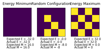
At absolute 0 the system will adapt the lowest energy configuration thus all spins will be parallel. This will give a magnetisation $M = 1000$

Calculating the energy and magnetisation

Task 4 and Task 7

Code for the initial IsingLattice function and the Montecarlostep

import numpy as np

class IsingLattice:

    E = 0.0
    E2 = 0.0
    M = 0.0
    M2 = 0.0

    n_cycles = 0

    def __init__(self, n_rows, n_cols):
        self.n_rows = n_rows
        self.n_cols = n_cols
        self.lattice = np.random.choice([-1,1], size=(n_rows, n_cols))

    def energy(self):
        "Return the total energy of the current lattice configuration."
        sumpart=0
        for i in range(self.n_rows):
            i1 = (i+1)%(self.n_rows)
            i2 = (i-1)%(self.n_rows)
            for ic in range(self.n_cols):
                ic1 = (ic+1)%(self.n_cols)
                ic2 = (ic-1)%(self.n_cols)
                sumpart = sumpart + self.lattice[i][ic] * self.lattice[i1][ic]
                sumpart = sumpart + self.lattice[i][ic] * self.lattice[i2][ic]
                sumpart = sumpart + self.lattice[i][ic] * self.lattice[i][ic1]
                sumpart = sumpart + self.lattice[i][ic] * self.lattice[i][ic2]
        energy = (-0.5)*sumpart
        return energy
    def magnetisation(self):
        "Return the total magnetisation of the current lattice configuration."
        sumspin = 0
        for i in self.lattice:
            for j in i:
                sumspin = sumspin+j
        magnetisation=sumspin
        return magnetisation

    def montecarlostep(self, T):
        # complete this function so that it performs a single Monte Carlo step
        energy = self.energy()
        #the following two lines will select the coordinates of the random spin for you
        random_i = np.random.choice(range(0, self.n_rows))
        random_j = np.random.choice(range(0, self.n_cols))
        #the following line will choose a random number in the rang e[0,1) for you
        random_number = np.random.random()
        #change spin of random number
        self.lattice[random_i,random_j] = -self.lattice[random_i,random_j]
        #find delta E
        newe=self.energy()
        deltae=newe-energy
        #determine whether new values can be accepted straigth away, no else function needed as the values are already changed
        if deltae > 0:
            expocalc=np.exp(-deltae/T)
            if random_number>expocalc:
			    #change lattice back as it below R
                self.lattice[random_i,random_j] = -self.lattice[random_i,random_j]
        energy=self.energy()
        magnetisation=self.magnetisation()
		#summations of values
        self.n_cycles=self.n_cycles+1
        self.E += self.energy()
        self.E2 += self.energy()**2
        self.M += self.magnetisation()
        self.M2 += self.magnetisation()**2
        
        return energy,magnetisation
        
        
    def statistics(self):
        Eav = self.E/self.n_cycles
        E2av = self.E2/self.n_cycles
        Mav = self.M/self.n_cycles
        M2av = self.M2/self.n_cycles
        # complete this function so that it calculates the correct values for the averages of E, E*E (E2), M, M*M (M2), and returns them
        return Eav,E2av,Mav,M2av

Task 5

Introduction to Monte Carlo simulation

Task 6

$n u m b e r (c o n f i g u r a t i o n s) = 2^{100} = 1.26765061 0^{30}$ So the time it takes is: $\frac{2^{n}}{1 0^{9} s^{- 1}} = 1.2676506 * 1 0^{21} s = 4.0196937 * 1 0^{13} y e a r s$

It would take $4.020 * 1 0^{13}$ years to get a single value of ${⟨ M ⟩}_{T}$ .

Task 8

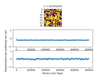
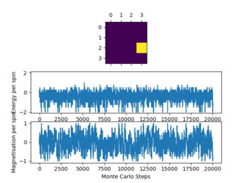
Below $T_{c}$ the thermal energy isn't great enough to flip spins readily, therefore the lowest energy state dominates over the entropy. If the temperature increases above the curie temperature the entropy dominates and no spontaneous magnetization occurs. Therefore we expect $⟨ M ⟩ \neq 0$

Figure 2: Monte Carlo simulation until equilibrium was reached

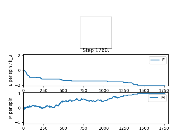
output of statistics file: Averaged quantities:

E = -1.47240896359

E*E = 2.32102153361

M = 0.569695378151

M*M = 0.43897551208

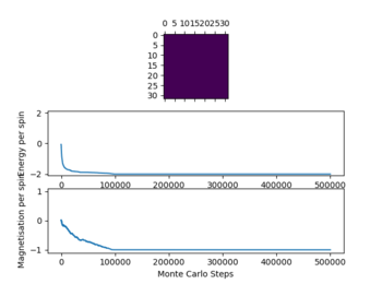
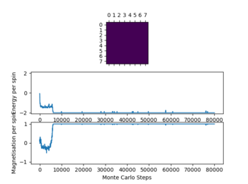
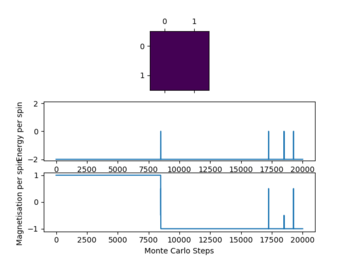
In the figure 2 the system reaches equilibrium at the lowest energy state as all spins align, therefore the system is at the lowest energy. Due to the small temperature the entropy doesn't dominate or contribute.

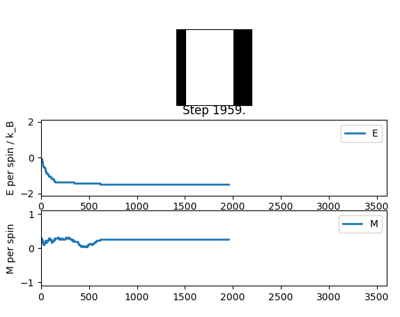
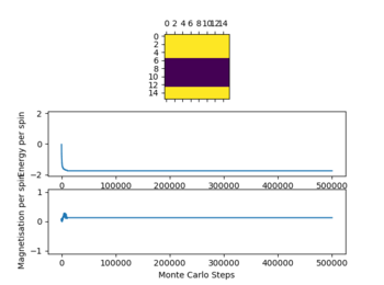
Figure 3: Monte Carlo simulation until a metastable equilibrium was reached

output of statistics file:

Averaged quantities:

E = -1.43791592724

E*E = 2.10344283773

M = 0.233543145519

M*M = 0.0570023950477

Even thou the system doesn't change in energy anymore it hasn't reached equilibrium, this is due to the fact that it is in the metastable region, where the simulation is at a local minimum and therefore doesn't change anymore as not enough energy is available to flip spins enough to overcome the energy barrier to the global minimum.

Accelerating the code

Task 10

Code of the accelerated function:

import numpy as np

class IsingLattice:

    E = 0.0
    E2 = 0.0
    M = 0.0
    M2 = 0.0

    n_cycles = 0

    def __init__(self, n_rows, n_cols):
        self.n_rows = n_rows
        self.n_cols = n_cols
        self.lattice = np.random.choice([-1,1], size=(n_rows, n_cols))

    def energy(self):
        "Return the total energy of the current lattice configuration."
        colums1=np.multiply(self.lattice,np.roll(self.lattice,1,axis=1))
        rows1=np.multiply(self.lattice,np.roll(self.lattice,1,axis=0))
        sumpart=np.sum(colums1)+np.sum(rows1)
        energy = (-1)*sumpart
        return energy
    def magnetisation(self):
        "Return the total magnetisation of the current lattice configuration."
        magnetisation = np.sum(self.lattice)
        return magnetisation

    def montecarlostep(self, T):
        # complete this function so that it performs a single Monte Carlo step
        energy = self.energy()
        #the following two lines will select the coordinates of the random spin for you
        random_i = np.random.choice(range(0, self.n_rows))
        random_j = np.random.choice(range(0, self.n_cols))
        #the following line will choose a random number in the rang e[0,1) for you
        random_number = np.random.random()
        #change spin of random number
        self.lattice[random_i,random_j] = -self.lattice[random_i,random_j]
        #find delta E
        newe=self.energy()
        deltae=newe-energy
        #determine whether new values can be accepted straigth away, no else function needed as the values are already changed
        if deltae > 0:
            expocalc=np.exp(-deltae/T)
            if random_number>expocalc:
                #change lattice back as it below R
                self.lattice[random_i,random_j] = -self.lattice[random_i,random_j]
        energy=self.energy()
        magnetisation=self.magnetisation()
        #summations of values
        self.n_cycles=self.n_cycles+1
        if self.n_cycles >0:
            self.E += self.energy()
            self.E2 += self.energy()**2
            self.M += self.magnetisation()
            self.M2 += self.magnetisation()**2
        return energy,magnetisation
        
        
    def statistics(self):
        Eav = self.E/(self.n_cycles-0)
        E2av = self.E2/(self.n_cycles-0)
        Mav = self.M/(self.n_cycles-0)
        M2av = self.M2/(self.n_cycles-0)
        cycles=self.n_cycles
        # complete this function so that it calculates the correct values for the averages of E, E*E (E2), M, M*M (M2), and returns them
        return Eav,E2av,Mav,M2av,cycles

Task 9 and Task 11

Before accelerating the simulation to run 2000 Monte Carlo steps took 14.90211159 seconds on average of 8 repeats with a standard deviation of 0.10146431 seconds. After acceleration it takes on an average of 8 repeats 0.449982787 seconds to run 2000 Monte Carlo steps with a standard deviation of 0.008642247 seconds.

The effect of temperature

Task 12 and Task 14

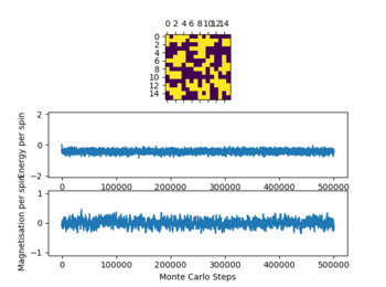
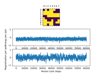
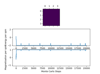
For all lattice sizes timesteps at T=0.25, T= 1 and T= 5 were recorded to show the equilibrium structure at these points.

Figure 4: Graphs at chosen number of steps at different temperatures for different lattice
Lattice	Number of steps	Number of steps ignored
32x32	500000	200000
16x16	500000	200000
8x8	80000	20000
4x4	20000	5000
2x2	20000	5000

In the table (Figure 4) above the ILfinalframe graphs are shown at the timestep chosen alongside the temperatures the simulations were run. Due to the data obtained a number of 80000 steps was chosen ignoring the first 20000 steps. This was done as with increasing temperature (while $T < T_{C}$ ) the simulation needs more time to reach equilibrium as seen above. This effect becomes more pronounced with increasing T. This occurs due to the increased influence of the entropy upon the energy as it is T dependent, which give a lot of local minima when approaching the Curie temperature. This effect can especially be observed in the graphs of the 32x32 lattice. 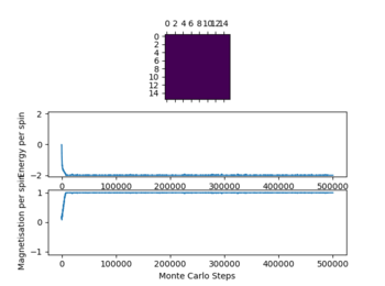Not all simulations reach the global minimum especially at lower temperatures (e.g 16x16 lattice at T=0.25), this occurs as the simulations reaches a local energy minimum with a thermal energy that is too low to overcome an energy barrier between this local minimum and the global minimum. For all lattice sizes the averages were only recorded once the system reached equilibrium, to ensure that this is the case also for higher temperatures above 1 the steps ignored were significantly larger than the values seen when the reaction reaches equilibrium.

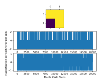
The graphs in figure 4 also show the significant effect of lattice size upon the magnetization and energy values changes. For the 2x2 lattice a change in flip can cause the system to flip magnetization as seen in one of the graphs. Note that the magnitude of the magnetization is important no the sign. Once the magnetization reaches its maximum magnitude the system is at equilibrium as all spins are aligned which gives the biggest magnetic moment.

Task 13 and task 14

Figure 5: Graphs of the Energy error bars
Lattice	Error bars of the mean Variance in Energy at equilibrium	Error bars of the repeats
32x32
16x16
8x8
4x4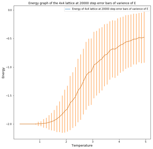
2x2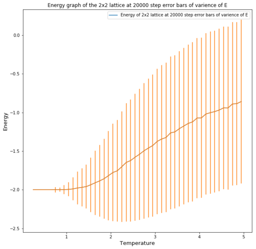

Figure 5: Graphs of the Magnetization error bars
Lattice	Error bars of the mean Variance in Magnetization at equilibrium	Error bars of the repeats
32x32
16x16
8x8
4x4
2x2

Figures 4 and 5 show the effect of the lattice size on the energy per spin and the accuracy of the repeats. One can see that for the energy the error obtained for the energy value at equilibrium is much greater the greater the temperature. This occurs as a higher thermal energy leads to more possible energy states as entropy place a big factor in the energy. The error also decreases significantly with increasing lattice size, this is due to the fact that for a small lattice, flipping one spin causes a large fluctuation in energy, therefore the error is very pronounced, especially at high temperatures where spins flip constantly.

The energy graphs also show that increasing the lattice size makes the phase transition more pronounced and more $δ$ function like.

Determining the heat capacity

Task 15

$C = d ⟨ E ⟩ / d T$

$⟨ E ⟩ = \sum_{i} E_{i} P_{i} = \frac{1}{Z} \sum_{i} E_{i} e^{- β * E_{i}}$

with

$β = \frac{1}{k_{B} T} a n d Z = \sum_{i} e^{- β * E_{i}}$

Thererfore

$\frac{1}{Z} \sum_{i} E_{i} e^{- β * E_{i}} = - \frac{1}{Z} \frac{d Z}{d β}$

$⟨ E^{2} ⟩ = \frac{1}{Z} \frac{d^{2} Z}{d β^{2}}$

$⟨ E^{2} ⟩ - {⟨ E ⟩}^{2} = \frac{1}{d β} (\frac{1}{Z} \frac{d Z}{d β}) = - \frac{1}{d β} ⟨ E ⟩$

$\frac{1}{d T} = \frac{1}{d β} * \frac{d β}{d T}$

$\frac{d β}{d T} = - k T^{2}$

$\frac{d ⟨ E ⟩}{d β} = k T^{2} \frac{d ⟨ E ⟩}{d T}$

$\frac{d ⟨ E ⟩}{d T} = C$

$C = \frac{⟨ E^{2} ⟩ - {⟨ E ⟩}^{2}}{k T^{2}}$

as

$⟨ E^{2} ⟩ - {⟨ E ⟩}^{2} = V a r [E]$

Therefore:

$C = \frac{V a r [E]}{k T^{2}}$

Task 16

Figure 6: Heatcapacity for the mean of all lattice sizes

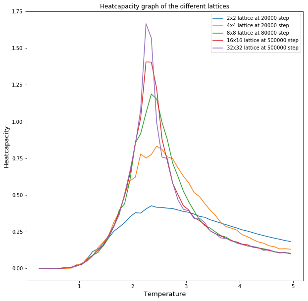
In figure 6 one can see all of the heatcapacities of the different Lattice sizes simulated using the code above. It can be seen that the peak of $C_{V}$ shifts left and increases with increasing lattice size. The heatcapacity should diverge at the curie temperature, however because we don't use an infinite lattice our heatcapacities don't diverge but reach a peak.

Locating the Curie temperature

Task 17

Figure 7: Comparison of C++ data and own calculated data for the 16x16 lattice

In figure 7 one can see the difference in the heatcapacity of the C++ data against the one simulated in this experiment. It can be seen that the data is very different around the peak, which suggests that around it the temperature step chosen in the simulation(0.1) was to great in that region. The rest of the plot fits with the C++ data. In future experiments one should decrease the temperature step around the curie temperature to ensure a better fit.

Task 18

Figure 8: Polyfit at full range of own simulated 8x8 lattice

Task 19

Figure 9: Polyfit with range restricted around peak of own simulated 8x8 lattice

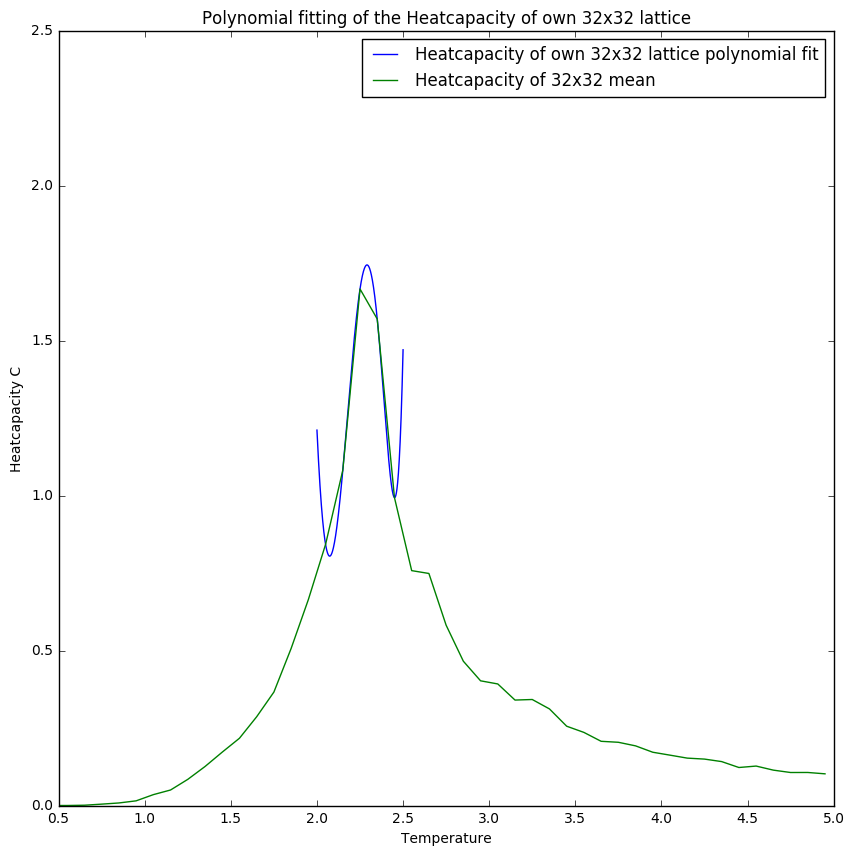
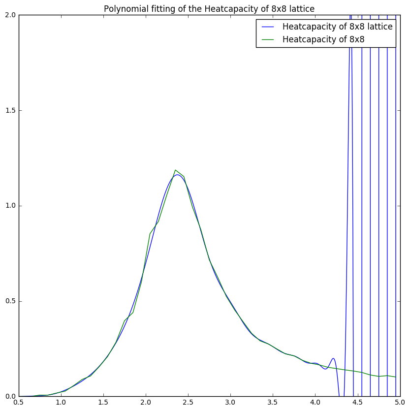
Comparing figures 8 and 9 one can see the importance of selecting the right range for fits as it gives a more reliable fit. This is especially illustrated in figure 10 where the polyfit is much more like the plot obtained from the C++ data.

Figure 10: Comparison of accuracy of Polyfit with 2x2 lattice against C++ data

Figure 11: Comparison of accuracy of Polyfit with 32x32 lattice against C++ data

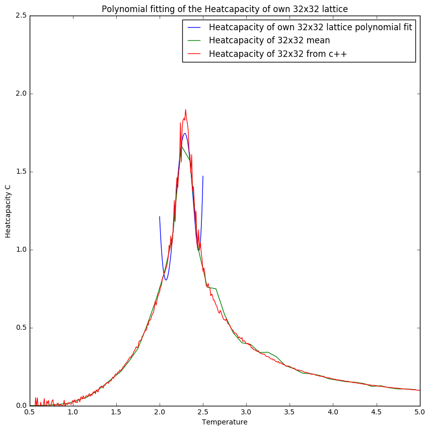
Figures 10 and 11 show that with increasing lattice size the simulation becomes less accurate for the heatcapacity compared to the C++ plots. This could be due to the fact that the heatcapacity at higher lattice sizes becomes more like a $δ$ function which means that the a small temperature step becomes more significant.

Task 20

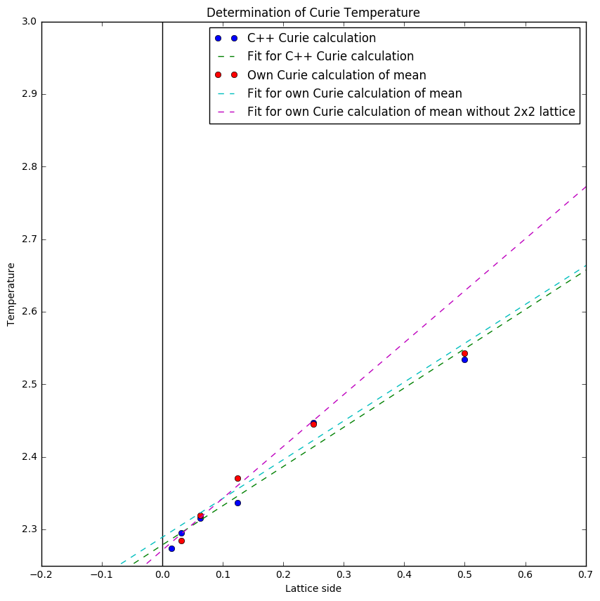
Figure 12: Plotted graph to find Curie Temperature

Figure 12 shows the curie temperatures obtained when plotting peak of the heatcapacity against 1 over the lattice size. The intercepts at 0 give the respective curie temperatures:

Own Curie temperature calculation:2.28887220375

C++ Curie temperature calculation: 2.2782708112437811

Selected range of own Curie temperature calculation: 2.2710319004347821

literature value: 2.269^[1] (Note the literature value is the exact solution to the 2D IsingLattice model calculated by Onsager)

One can see that the C++ data is more accurate than the simulations done in this experiment. However once the 2x2 lattice heatcapacity was excluded the value of the Curie Temperature became much more accurate. This could be due to the large error associated to the 2x2 Lattice heatcapacity as can be seen in figure 13. Considering how close the value of the simulation is to the actual value shows the effectiveness of this simulation. The biggest source of error is the limited lattice sizes and the temperature step being to great in the critical region.

Figure 13: Graphs of the heatcapacity error bars
Lattice	Error bars of the heatcapacity of repeats at equilibrium
32x32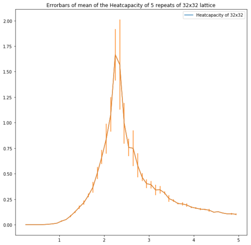
16x16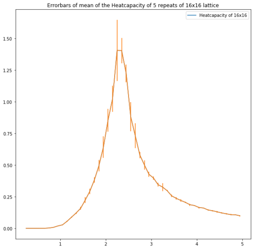
8x8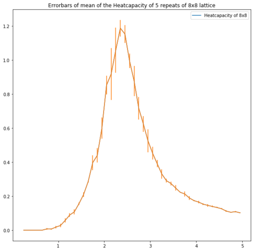
4x4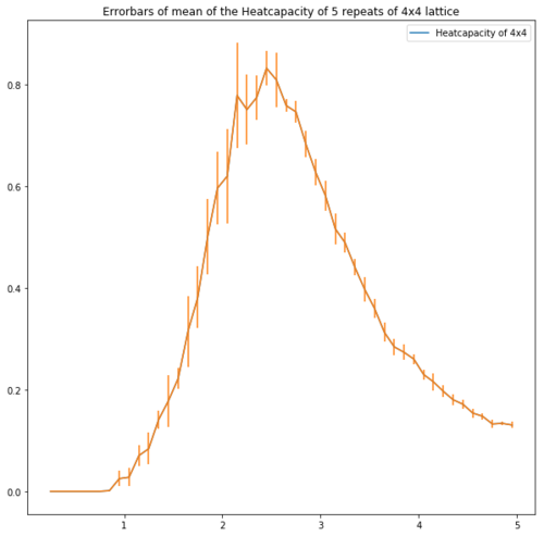
2x2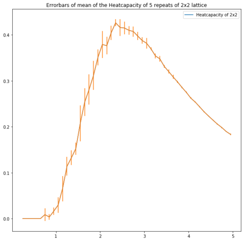

Figure 13 shows the error bars of the heatcapacities. These show that for the bigger lattices the error is high around the peak which supports the idea of repeating with a smaller temperature step.

Functions for plotting

Task 13 and 14

def make_plotenergy(dataname,Title,size):
    T=dataname[:,0]
    E=dataname[:,1]
    E2=dataname[:,2]
    Eps=E/(size**2)
    Eps2=E2/(size**4)
    VarE=(Eps2-(Eps)**2)
    #sterrorb=(VarE/steps)**0.5
    sterrorb=VarE**0.5
    
    figsize(10,10)
    
    title("Energy graph of the "+Title)
    
    xlabel("Temperature",fontsize=13)
    ylabel("Energy",fontsize=13)
    plot(T,E/(size**2),label="Energy of "+Title)
    errorbar(T, E/(size**2), xerr=0, yerr=sterrorb)
    legend()
    return

def make_plotenergydifferr(dataname,dataerror,Title,size):
    T=dataname[:,0]
    E=dataname[:,1]
    E2=dataname[:,2]
    Eps=E/(size**2)
    Eps2=E2/(size**4)
    sterrorb=dataerror
    
    figsize(10,10)
    
    title("Energy graph of the "+Title)
    
    xlabel("Temperature",fontsize=13)
    ylabel("Energy",fontsize=13)
    plot(T,E/(size**2),label="Energy of "+Title)
    errorbar(T, E/(size**2), xerr=0, yerr=sterrorb)
    legend()
    return

def make_plotmag(dataname,Title):
    T=dataname[:,0]
    M=dataname[:,3]
    M2=dataname[:,4]
    
    VarM=(M2-(M)**2)
    sterrorb=(VarM)**0.5
    
    figsize(10,10)
    
    title("Magnetisation graph of the "+Title)
    
    xlabel("Temperature",fontsize=13)
    ylabel("Magnetisation",fontsize=13)
    plot(T,M,label="Magnetisation of "+Title)
    errorbar(T, M, xerr=0, yerr=sterrorb)
    legend()
    return

def make_plotmagdifferr(dataname,dataerror,Title,size):
    T=dataname[:,0]
    M=dataname[:,3]
    M2=dataname[:,4]
    Mps=M/(size**2)
    Mps2=M2/(size**4)
    sterrorb=dataerror
    
    figsize(10,10)
    
    title("Magnetisation graph of the "+Title)
    
    xlabel("Temperature",fontsize=13)
    ylabel("Magnetisation",fontsize=13)
    plot(T,M/(size**2),label="Energy of "+Title)
    errorbar(T, M/(size**2), xerr=0, yerr=sterrorb)
    legend()
    return

def support_plotenergy(dataname,Title):
    T=dataname[:,0]
    E=dataname[:,1]
    
    
    VarE=(E2-(E)**2)
    #sterrorb=(VarE/steps)**0.5
    sterrorb=VarE**0.5
    
    
    figsize(10,10)
    
    
    plot(T,E,label="Energy of "+Title)
    errorbar(T, E, xerr=0, yerr=sterrorb)
    legend()
    return

def support_plotenergywithouteer(dataname,Title,size):
    T=dataname[:,0]
    E=dataname[:,1]
    
    
    
    
    
    figsize(10,10)
    
    
    plot(T,E/(size**2),label="Energy of "+Title)
    legend()
    return

def support_plotmag(dataname,Title):
    T=dataname[:,0]
    M=dataname[:,3]
    
    
    M2=dataname[:,4]
    
    VarM=(M2-(M)**2)
    sterrorb=(VarM)**0.5
    
    
    figsize(10,10)
    
    
    plot(T,M,label="Magnetisation of "+Title)
    errorbar(T, M, xerr=0, yerr=sterrorb)
    legend()
    return

Task 16

def make_plotheatcap(dataname,Title,size):
    T=dataname[:,0]
    E=dataname[:,1]
    E2=dataname[:,2]
    
    heatcap=(E2-(E)**2)/((size**2)*(T**2))
    figsize(10,10)
    title("Heatcapacity graph of the different lattices")
    
    xlabel("Temperature",fontsize=13)
    ylabel("Heatcapacity",fontsize=13)
    plot(T,heatcap,label=Title)
    #legend()
    return

def support_plotheatcap(dataname,Title,size):
    T=dataname[:,0]
    E=dataname[:,1]
    E2=dataname[:,2]
    heatcap=(E2-(E)**2)/((size**2)*(T**2))
    figsize(10,10)
    
    plot(T,heatcap,label=Title)
    legend()
    return

Task 17

def support_plotheatcapc(dataname,Title):
    T=dataname[:,0]
    E=dataname[:,1]
    E2=dataname[:,2]
    C=dataname[:,5]
    k=1.38*10**(-23)
    
    heatcap=(E2-(E)**2)/((T**2))
    figsize(10,10)
    
    plot(T,C,label="Heatcapacity of "+Title)
    legend()
    return

Task 18 and 19

def make_plotheatcapofC(dataname,deg,Title,region1,region2,xlimits,ylimits):
    T = dataname[:,0] #get the first column
    C = dataname[:,5] # get the second column

    #first we fit the polynomial to the data
    
    Tmin = region1 #for example
    Tmax = region2 #for example

    selection = np.logical_and(T > Tmin, T < Tmax) #choose only those rows where both conditions are true
    peak_T_values = T[selection]
    peak_C_values = C[selection]
    
    fit = np.polyfit(peak_T_values, peak_C_values, deg) # fit a third order polynomial
    
    #now we generate interpolated values of the fitted polynomial over the range of our function
    T_range = np.linspace(Tmin, Tmax, 1000) #generate 1000 evenly spaced points between T_min and T_max
    fitted_C_values = np.polyval(fit, T_range) # use the fit object to generate the corresponding values of C
    
    figsize(10,10)
    
    ylabel("Heatcapacity C")
    xlabel("Temperature")
    
    
    title("Polynomial fitting of the Heatcapacity of "+Title+" lattice")
    xlim(0.5,xlimits)
    ylim(0,ylimits)
    plot(T_range,fitted_C_values,label="Heatcapacity of "+Title+" lattice polynomial fit")
    
    Cmax = np.max(fitted_C_values)
    Tmax = T_range[fitted_C_values == Cmax]
    return Cmax,Tmax

def make_plotheatcapofown(dataname,size,deg,Title,region1,region2,xlimits,ylimits,range1,range2):
    T = dataname[:,0] #get the first column
    E=dataname[:,1]
    E2=dataname[:,2]
    #first we fit the polynomial to the data
    C=(E2-(E)**2)/((size**2)*(T**2))

    
    Tmin = region1 #for example
    Tmax = region2 #for example

    selection = np.logical_and(T > Tmin, T < Tmax) #choose only those rows where both conditions are true
    peak_T_values = T[selection]
    peak_C_values = C[selection]
    
    fit = np.polyfit(peak_T_values, peak_C_values, deg) # fit a third order polynomial
    
    #now we generate interpolated values of the fitted polynomial over the range of our function
    T_range = np.linspace(Tmin, Tmax, 1000) #generate 1000 evenly spaced points between T_min and T_max
    fitted_C_values = np.polyval(fit, T_range) # use the fit object to generate the corresponding values of C
    
    figsize(10,10)
    
    ylabel("Heatcapacity C")
    xlabel("Temperature")
    
    title("Polynomial fitting of the Heatcapacity of "+Title+" lattice")
    xlim(0.5,xlimits)
    ylim(0,ylimits)
    plot(T_range,fitted_C_values,label="Heatcapacity of "+Title+" lattice polynomial fit")
    
    Cmax = np.max(fitted_C_values[range1:range2])
    Tmax = T_range[fitted_C_values == Cmax]
    return Cmax,Tmax

Task 20

figsize(10,10)

ylim(2.25,3)
xlim(-0.2,0.7)
owncuriefit=polyfit(owncurieviagrad[:,0], owncurieviagrad[:,1],1)
precalccuriefit=polyfit(precalccurieviagrad[:,0], precalccurieviagrad[:,1],1)
owncuriefitofmeansel=polyfit(owncurieviagradofmean[1:,0], owncurieviagradofmean[1:,1],1)
owncuriefitofmean=polyfit(owncurieviagradofmean[:,0], owncurieviagradofmean[:,1],1)

x=arange(-1,5,0.01)

title("Determination of Curie Temperature")

xlabel("Lattice side")
ylabel("Temperature")


plot(x*0,x,linestyle="-",color="black")
#plot(owncurieviagrad[:,0],owncurieviagrad[:,1],marker="o",linestyle="",label="Own Curie calculation")
plot(precalccurieviagrad[:,0],precalccurieviagrad[:,1],marker="o",linestyle="",label="C++ Curie calculation")
#plot(x,x*owncuriefit[0]+owncuriefit[1],linestyle="--",label="Fit for own Curie calculation")
plot(x,x*precalccuriefit[0]+precalccuriefit[1],linestyle="--",label="Fit for C++ Curie calculation")
plot(owncurieviagradofmean[:,0],owncurieviagradofmean[:,1],marker="o",linestyle="",label="Own Curie calculation of mean")
plot(x,x*owncuriefitofmean[0]+owncuriefitofmean[1],linestyle="--",label="Fit for own Curie calculation of mean")

#plot(owncurieviagradofmean[0:-1,0],owncurieviagradofmean[0:-1,1],marker="o",linestyle="",label="Own Curie calculation of mean without 2x2 lattice")
plot(x,x*owncuriefitofmeansel[0]+owncuriefitofmeansel[1],linestyle="--",label="Fit for own Curie calculation of mean without 2x2 lattice")

legend()

references

<references> ^[1]

↑ ^1.0 ^1.1 L. Onsager, Phys. Rev. 65, 117 (1944).

[curi-1] 1.0 ^1.1 L. Onsager, Phys. Rev. 65, 117 (1944).

[1]