Rep:Jmt12ls

Simulation of a simple liquid

Introduction

Molecular dynamics is an important way to simulate liquids. The interactions between atoms for a specific ensemble in a liquid are studied, over a given time. A number of approximations must be made so that the computations are possible. It is assumed that the particles behave as classical particles and they are subjected to a force which originates from the interactions of the other particles. This force is the reason that the particles accelerate.

Introduction to molecular dynamics simulation

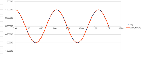
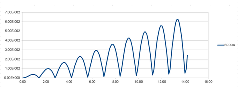
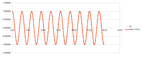
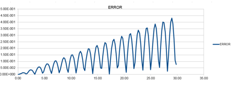
The Harmonic oscillator was modeled using the velocity Verlet algorithm and the following graphs were produced from this. The first graph was made by plotting the value of the classical solution for the harmonic oscilator against time, from 0 seconds to 14.2 seconds. The second graph was an error plot of the absolute difference between the approximate values from the velocity Verlet solution and the values obtained from the harmonic oscillator equation. The third graph was produced by calculating the sum of the potential and kinetic energy for the velocity Verlet solution at each time. The values used in these calculations were; k = 1.00, mass = 1.00, $\varphi$ = 0.00, A = 1.00, $\omega$ = 1.00 and a timestep of 0.100.

The positions at a time, $t$ were calculated by use of the equation ;$x\left(t\right)=A\cos (\omega t+\varphi )$.

The energies were calculated by using the equation; $E=\frac{1}{2}m{v}^2+\frac{1}{2}k{x}^2$

Graph 1 - Analytical

Graph 2 - Error

Graph 3 - Total energy

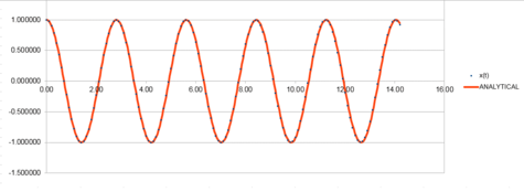
In the tables below, everything was calculated in the same way as above, however, this time, the value of k was increased from 1.00 to 5.00. It is evident by comparison that increasing the value of the force constant (k) has increased the frequency of vibrations. This is because, it is known that;

$\omega =\sqrt{\frac{k}{\mu }}$

so by looking at the equation above, it is obvious that if the force constant, $k$ is increased, this will therefore also cause the frequency, $\omega$ to also increase.

Graph 4 - Analytical (increased k)

Graph 5 - Error (increased k)

Graph 6 - Total energy (increased k)

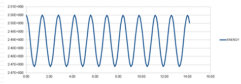The equation $\omega =\sqrt{\frac{k}{\mu }}$ also shows that the frequency will also increase if all of the values are kept the same apart from if the mass is decreased. This can be seen in the tables below, where the mass was decreased from 1.00 to 0.25.

Graph 4a - Analytical (decreased mass)

Graph 5a - Error (decreased mass)

Graph 6a - Total energy (decreased mass)

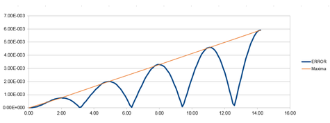
Graph 7 was produced by plotting each maxima value for the error plot against time.

Graph 7 - Error maxima

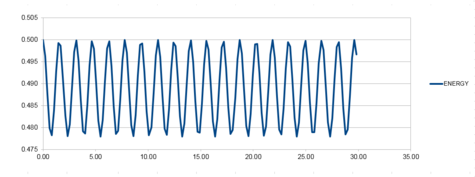
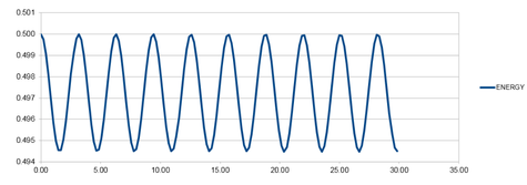
So that the difference in energy does not change by more than 1%, the largest value of the timestep would need to be 0.200. This was calculated because if the total energy at its highest is 0.500, then the total energy at its lowest must not be smaller than 0.495. The value of the timestep was changed and the difference between the energy minima and maxima was calculated. The graph for the energy that was produced for this timestep value can be seen in graph 8, below.

Graph 8 - Energy graph with total energy difference at 1%

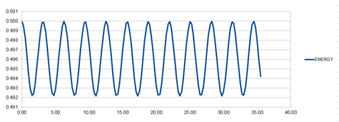
A larger value for the timestep was inserted to show that the overall energy did change by more than 0.495 when the timestep was increased past 0.200. The graph that was produced from a timestep of 0.250 shown below as graph 9. The lowest value for the total energy at this timestep is 0.492.

Graph 9 - Energy difference above 1%

It is important to monitor the total energy of a physical system when modelling its behaviour numerically so that you know that the law of conservation of energy has been obeyed. If it has not, then the simulation will not accurately reflect a real system.

Atomic Forces

The Lennard-Jones potential is used to simulate the interactions between a pair of atoms in a simple liquid. For a single Lennard-Jones interaction,

$\varphi \left(r\right)=4ϵ(\frac{{\sigma }^{12}}{r^{12}}-\frac{{\sigma }^6}{r^6})$

When the potential energy is equal to zero, the separation $r_0$ is;

$4ϵ(\frac{{\sigma }^{12}}{r^{12}}-\frac{{\sigma }^6}{r^6})=0$

$(\frac{{\sigma }^{12}}{r^{12}}-\frac{{\sigma }^6}{r^6})=0$

$\frac{{\sigma }^{12}}{r^{12}}=\frac{{\sigma }^6}{r^6}$

$\frac{{\sigma }^{12}}{{\sigma }^6}=\frac{r^{12}}{r^6}$

${\sigma }^6=r^6$

$\sigma =r$

and therefore $r_0=0$

At this separation the force is calculated from

${\mathbf{F}}_i=-\frac{\mathrm{d}U\left({\mathbf{r}}^N\right)}{\mathrm{d}{\mathbf{r}}_i}$

If this value for $r_{eq}$ is substituted into

therefore

${\mathbf{F}}_i=-4ϵ(\frac{-12{\sigma }^{12}}{r^{13}}-\frac{-6{\sigma }^6}{r^7})$

${\mathbf{F}}_i=4ϵ(\frac{12{\sigma }^{12}}{r^{13}}-\frac{6{\sigma }^6}{r^7})$

If $r=\sigma$ then

${\mathbf{F}}_i=4ϵ(\frac{12{\sigma }^{12}}{{\sigma }^{13}}-\frac{6{\sigma }^6}{{\sigma }^7})$

${\mathbf{F}}_i=4ϵ(\frac{12}{\sigma }-\frac{6}{\sigma })$

${\mathbf{F}}_i=4ϵ\left(\frac{6}{\sigma }\right)$

At equilibrium, we are at the bottom of the curve and the derivative of the Lennard-Jones potential and also the force can be set to equal 0. The value of $r$ will then be equal to the equilibrium separation, $r_{eq}$, as below:

$4ϵ(\frac{12{\sigma }^{12}}{r^{13}}-\frac{6{\sigma }^6}{r^7})=0$

$4ϵ\left(\frac{12{\sigma }^{12}}{r^{13}}\right)=4ϵ\left(\frac{6{\sigma }^6}{r^7}\right)$

$\frac{48ϵ{\sigma }^{12}}{r^{13}}=\frac{24ϵ{\sigma }^6}{r^7}$

$\frac{48ϵ{\sigma }^{12}}{24ϵ{\sigma }^6}=\frac{r^{13}}{r^7}$

$2{\sigma }^6=r^6$

$r_{eq}{=}^6\sqrt{2}\sigma$

The well depth, $\varphi (r_{eq})$, can be found by substituting this value for $r_{eq}$ into

$\varphi =4ϵ(\frac{{\sigma }^{12}}{r^{12}}-\frac{{\sigma }^6}{r^6})$

To give

$\varphi (r_{eq})=4ϵ(\frac{{\sigma }^{12}}{{(}^6\sqrt{2}\sigma {)}^{12}}-\frac{{\sigma }^6}{{(}^6\sqrt{2}\sigma {)}^6})$

$\varphi (r_{eq})=4ϵ(\frac{{\sigma }^{12}}{4\sigma }-\frac{{\sigma }^6}{2\sigma })$

$\varphi (r_{eq})=4ϵ(\frac{{\sigma }^{12}}{4{\sigma }^{12}}-\frac{{\sigma }^6}{2{\sigma }^6})$

$\varphi (r_{eq})=4ϵ(\frac{1}{4}-\frac{1}{2})$

$\varphi (r_{eq})=(\frac{4ϵ}{4}-\frac{4ϵ}{2})$

$\varphi (r_{eq})=-ϵ$

When $\sigma =ϵ=1.0$;

$\varphi \left(r\right)=4(\frac{1}{r^{12}}-\frac{1}{r^6})$

$\varphi \left(r\right)=4(r^{-12}-r^{-6})$

$\underset{x}{\overset{\mathrm{\infty }}{\int }}\varphi \left(r\right)\mathrm{d}r=4{(\frac{-r^{-11}}{11}+\frac{r^{-5}}{5})}_x^{\mathrm{\infty }}$

The below integrals were then evaluated;

• $\underset{2\sigma }{\overset{\mathrm{\infty }}{\int }}\varphi \left(r\right)\mathrm{d}r$

$=-0.0248$

• $\underset{2.5\sigma }{\overset{\mathrm{\infty }}{\int }}\varphi \left(r\right)\mathrm{d}r$

$=-8.17\times 10^{-3}$

• $\underset{3\sigma }{\overset{\mathrm{\infty }}{\int }}\varphi \left(r\right)\mathrm{d}r$

$=-3.29\times 10^{-3}$

Periodic boundary conditions

Under standard conditions, in 1 ml of water;

$n=\frac{1}{18}=0.0555moles$

Therefore

$no.atoms=0.0555\times (6.022\times 10^{23})=3.345\times 10^{22}$ in 1ml

For 10000 atoms;

$n=\frac{10000}{6.022\times 10^{23}}=1.6606\times 10^{-20}moles$

$mass=moles\times molarmass=(1.6606\times 10^{-20})\times 18=2.989\times 10^{-19}g$

$volume=\frac{mass}{density}=\frac{2.989\times 10^{-19}}{1}$

$=2.989\times 10^{-19}c{m}^{-3}$

If an atom at position $(0.5,0.5,0.5)$ in a cubic simulation box which runs from $(0,0,0)to(1,1,1)$. In a single timestep, it moves along the vector $(0.7,0.6,0.2)$.

After the periodic boundary conditions have been applied, the atom would end up at position $(0.2,0.1,0.7)$.

Reduced units

When looking at the Lennard-Jones potential, reduced units are usually used instead of real units. This is done so that the values are more manageable.

The Lennard-Jones parameters for argon are $$\begin{gathered} \sigma =0.34\mathrm{n}\mathrm{m},ϵ \\ / \\ {k}_B=120\mathrm{K} \end{gathered}$$.

If the LJ cutoff is $r^{*}=3.2$, in real units this would be

$r^{*}=\frac{r}{\sigma }$

$3.2=\frac{r}{0.34}$

$r=1.088nm$

What is the well depth in $$\begin{gathered} {\mathrm{k}\mathrm{J} \\ \mathrm{m}\mathrm{o}\mathrm{l}}^{-1} \end{gathered}$$?

The well depth, $\varphi =-ϵ$

and because, from above;

$$\begin{gathered} ϵ \\ / \\ {k}_B=120\mathrm{K} \end{gathered}$$

Therefore

$$\begin{gathered} \varphi =\frac{-120\times \\ {k}_B\times N_A}{1000} \end{gathered}$$

$\varphi =-0.998kJ.mo{l}^{-1}$

The reduced temperature $T^{*}=1.5$ in real units is

$T^{*}=\frac{k_{B}T}{ϵ}$

and

$$\begin{gathered} ϵ \\ =120 \\ {k}_B \end{gathered}$$

therefore

$T^{*}=\frac{k_{B}T}{120k_B}$

$1.5=\frac{T}{120}$

$T=180K$

Equilibration

Creating the simulation box

For this, five different simulations were run using LAMMPS. Each simulation was run with a different timestep value; 0.001, 0.0025, 0.0075, 0.01 and 0.015.

It is easier to create starting points for the simulation if we are dealing with a crystal structure rather than if we are dealing with a liquid. This is because the crystal structure could simply be looked up but random starting points would have to be generated for a liquid. However, if atoms are given random starting coordinates then they may be have too strong a repulsion from each other, this means that they will be forced away from each other and cause issues in the simulation.

If the distance between the points of lattice is 1.07722 then the volume of the cube is equal to;

$1.07722^3=1.2500$

$\frac{numberofatoms}{volume}=density$

therefore,

$\frac{1}{1.2500}=0.8$

If we now look at a face centered cubic lattice, with a lattice point number density of 1.2 then, as there is a total of 4 whole atoms in the cube;

$\frac{numberofatoms}{density}=volume$

$\frac{4}{1.2}=3.333$

$Volume=3.333$ therefore the $length=3.333^{\frac{1}{3}}=1.494$

If we were to use the create_atoms command for 1000 units of the face centered cubic lattice then it would have created $4\times 1000=4000atoms$

Setting the properties of the atoms

The LAMMPS manual defines the following commands as:

• mass 1 1.0 - this command sets all atoms of type 1 (which is all of our atoms) to a mass of 1.0

• pair_style lj/cut 3.0 - this command computes pairwise interactions. These interactions are assessed within a specific boundary, or cut off point, in this case the cut off point is set as 3.0. lj in this command means Leonard Jones.

• pair_coeff * * 1.0 1.0 - this command is to define the pairwise force field coefficients between a pair(s) of atom types.

We are specifying ${\mathbf{x}}_i\left(0\right)$ and ${\mathbf{v}}_i\left(0\right)$ which means that the velocity Verlet algorithm is being used.

Running the simulation

In the code, the below is written:

### SPECIFY TIMESTEP ###
variable timestep equal 0.001
variable n_steps equal floor(100/${timestep})
variable n_steps equal floor(100/0.001)
timestep ${timestep}
timestep 0.001

### RUN SIMULATION ###
run ${n_steps}
run 100000

This section of the code is present because we want to tell LAMMPS that every time, after this code, it comes across ${timestep} we want it to replace it with 0.001, in this case.

We are not able to simply write:

timestep 0.001
run 100000

instead of writing the first command, above, because we want to keep the overall time the same and just change the timestep. The second, simpler code would change both the timestep and the total time of the simulation.

Visualising the trajectory

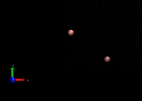
The trajectories can be viewed using the VMD programme as can be seen in figure 1, below.

Figure 1 - Representation of the atoms

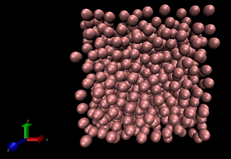
The periodic boundary conditions can also be visulaised using the VMD programme.

Figure 2 - Representation of two atoms

Checking equilibration

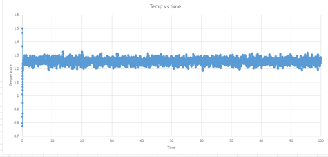
Here, the thermodynamic data will be used to see if the system has reached equilibrium. As can be seen from graphs 10, 11 and 12, below, the system does reach equilibrium. This is evident because, initially, there is a large change in the three graphs representing the energy, temperature and pressure. However, after this large change, the three variables then begin to fluctuate about the average, which must be the equilibrium state. It takes approximately 0.42 seconds by looking at the graphs.

Graph 10 - Energy vs time (0.001 timestep)

Graph 11 - Temperature vs time (0.001 timestep)

Graph 12 - Pressure vs time (0.001 timestep)

Graph 13 shows the difference in the energy over time for each of the five timesteps under analysis. A shorter timestep means that the calculated results will be closer to the experimental results, however, the shorter timestep also means that the measurements will have to take place over a shorter amount of time. This can be an issue if it is required that the calculations be run over a long period. As can be seen from graph 13 the timesteps with values of 0.001, 0.0025, 0.0075 and 0.01 all reach equilibrium. The data corresponding to the longest timestep of 0.015 shows the largest deviation from reality. This set of data does not reach an equilibrium and instead the the energy continues to rise, thus disobeying the law of conservation of energy. This timestep would therefore be the worst choice.

Graph 13 - Comparison of energy vs time for all timesteps

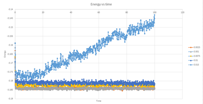
By looking at graph 14, it can be seen that the data series corresponding to the two smallest timestep values deviate the least from the average value whilst the data for the timestep values of 0.075 and 0.01 deviate noticeably more. It can be concluded that the largest timestep which still gives accurate results is the 0.0025 value.

Graph 14 - Comparison of energy vs time for all timesteps (zoomed in)

Running simulations under specific conditions

In this section, the simulations were modified so that the NpT (isobaric-isothermal) ensemble conditions were followed. The previous section simulated the liquid under microcanonical (NVE) ensemble conditions.

Ten simulations were run for this section. The timestep was set to 0.001 because then the most accurate results would be obtained. Five different temperatures were chosen. These temperatures needed to be higher than the critical temperature of T* = 1.5. The temperatures that were chosen were T = 1.6, 2.6, 3.6, 4.6, 5.6. Finally, two pressures needed to be chosen. These were chosen by looking at the average pressure from graph 12. The pressures that were chosen were p = 2.50 and 3.00.

Each of the five temperatures were run at each of the two pressures for a timestep of 0.001.

Thermostats and Barostats

In statistical thermodynamics, the equipartition theorem states that every degree of freedom for a system at equilibrium has an energy equal to $\frac{1}{2}{k}_{B}T$. As we are considering a system of $N$ atoms which each have three degrees of freedom, the following equation can be written:

$\frac{1}{2}\sum _i{m}_i{v}_i^2=\frac{3}{2}N{k}_{B}T(equation1)$

After every timestep, the kinetic energy can be calculated using equation 1. We use the left side of the equation and then divide this by $\frac{3}{2}N{k}_B$ so that $T$, the instantaneous temperature, can be calculated. We want this instantaneous temperature to equal the temperature that was specified in the script, the target temperature, $\mathfrak{𝔗}$. This can be achieved by multiplying each velocity by a constant, $\gamma$. This constant is calculated by solving equation 1 and equation 2.

$\frac{1}{2}\sum _i{m}_i{v}_i^2=\frac{3}{2}N{k}_{B}T(equation1)$

$\frac{1}{2}\sum _i{m}_i{\left(\gamma v_i\right)}^2=\frac{3}{2}N{k}_B\mathfrak{𝔗}(equation2)$

This can be done by dividing equation 2 by equation 1 to obtain:

$\frac{\frac{1}{2}\sum _i{m}_i{\left(\gamma v_i\right)}^2}{\frac{1}{2}\sum _i{m}_i{v}_i^2}=\frac{\frac{3}{2}N{k}_B\mathfrak{𝔗}}{\frac{3}{2}N{k}_{B}T}$

${\gamma }^2=\frac{\mathfrak{𝔗}}{T}$

Therefore

$\gamma =(\frac{\mathfrak{𝔗}}{T}{)}^{\frac{1}{2}}$

Examining the Input Script

fix aves all ave/time 100 1000 100000 v_dens v_temp v_press v_dens2 v_temp2 v_press2

The above line is present in the input script. This line tells LAMMPS to take an average of certain values over a certain number of timesteps. The order that the values are inserted is important.

The first value, which in this case is 100, corresponds to Nevery. This means that the values will be averaged every 100 timesteps.

The second value, 1000, corresponds to Nrepeat. This means that LAMMPS will use 1000 input values to calculate the averages.

The final value, 100000, corresponds to Nfreq. LAMMPS will therefore calculate averages every 100000 timesteps.

The amount of time that will be simulated is 100000.

Plotting the Equations of State

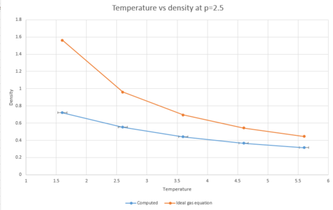
The density as a function of temperature was plotted for both of the chosen pressures.

Graph 15 - Density as a function of temperature at p=2.5

Graph 16 - Density as a function of temperature at p=3

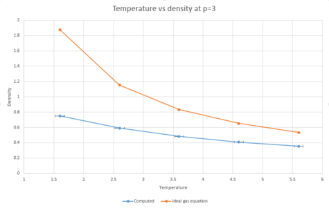As can be seen from the graphs, both of the plots of density as a function of temperature are higher for the plot using the density predicted by the ideal gas law than for the computed density. This is because the ideal gas equation assumes that the atoms do not interact with each other. This means that there would be less repulsion between atoms and they will therefore will not have to be as far away from each other as they would in reality. As;

$density=\frac{mass}{volume}$

and because the atoms are able to be closer together, the volume will be decreased due to the ideal gas law. From the equation above, then, by decreasing the volume, the density will have to increase as the mass is kept constant.

From the graphs, the higher the temperature is, the lower the density is. This is due to an increase in kinetic energy with rising temperature, meaning that the atoms will be further apart from each other and therefore the density will decrease.

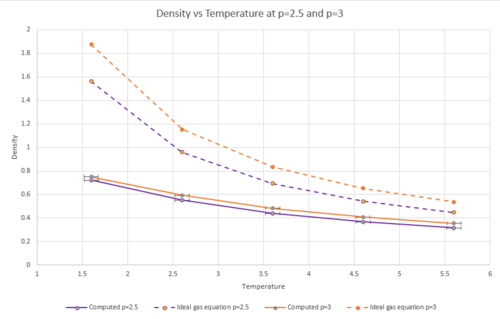
The data points for both pressures were plotted on the same axes to compare the deviation from the ideal gas equation plots at the two different pressures. The graph below shows that increasing the pressure leads to more deviations from the density predicted by the ideal gas equation. This can be explained because the ideal gas law ignores interactions with other atoms. At lower densities, in a real system, there will be fewer interactions taking place. This means that at lower densities, properties of a real system are more reflective of the same properties as predicted by the ideal gas law.

Density as a function of temperature at p=2.5, p=3

Calculating heat capacities using statistical physics

This section concentrated on the NVT ensemble. As the temperature is being held constant, in its equilibrium state, the energy must be fluctuating about an average value. These fluctuations about the average relate to the magnitude of the heat capacity according to the equation:

$C_V=\frac{\partial E}{\partial T}=\frac{\mathrm{V}\mathrm{a}\mathrm{r}\left[E\right]}{k_B{T}^2}=N^2\frac{⟨E^2⟩-{⟨E⟩}^2}{k_B{T}^2}$

The input files for this section were a modification of the file from the previous section.

Again, ten different simulations were run for this section, but this time in the density-temperature phase space.

The simulations were run at two densities of 0.2 and 0.8 and five temperatures of 2.0, 2.2, 2.4, 2.6 and 2.8. The graph below shoes a plot of $C_V$ as a function of temperature. An example of one of the input files used can be found here. This is for a temperature of 2.0 and a density of 0.2.

Graph 19 - Cv vs T for density of 0.2 and 0.8

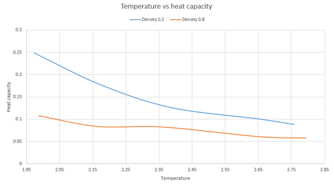
The below graph shows $C_V/V$ as a function of temperature. The volume was calculated by $\frac{numberofatoms}{density}=volume$. The number of atoms for both densities was 3375. This gave a volume of 16875 for the density of 0.2 and a volume of 4218 for the density of 0.8

Graph 20 - Cv/V vs T for density of 0.2 and 0.8

As can be seen from the above graph, as the temperature increases, the heat capacity per unit volume decreases. The simulation at the higher density has a larger heat capacity compared to the lower density one for the same temperature. The higher the density, the higher the number of atoms will be when we are looking at an equal volume. The heat capacity is an extensive property of the system. This means that as the size of the system increases, the heat capacity will also increase, which is supported by looking at the graph above.

Structural properties and the radial distribution function

The radial distribution function (RDF), $g(r)$, is a measure of density with respect to the distance from an atom. Using this function, the distance of the nearest neighbours of a certain atom can be calculated.

This journal . provided the phase diagram of the Leonard-Jones potential that was used to choose the pressures and temperatures of a solid, liquid and gas that the simulations in this sections were run with. The table below shows these differing values for the different phases.

	Solid	Liquid	Vapour
Temperature	1.2	1.15	1.15
Density	1.2	0.6	0.09

The results of the simulations of the Leonard-Jones system were then used in VMD to calculate $g(r)$ and $\int g(r)\mathrm{d}r$.

The RDFs of a (fcc) solid, a liquid and a vapour are shown on the same axis, for comparison, in graph 21, below.

Graph 21 - RDFs for solid, liquid and gas

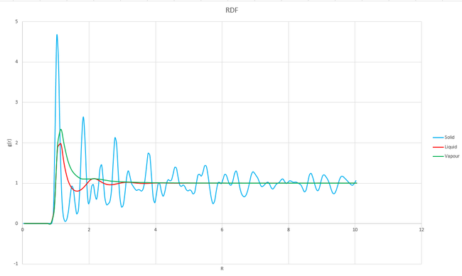
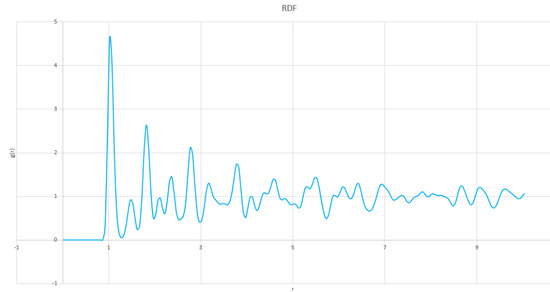
Graph 21 shows the probability of finding at atom at different distances with respect to another atom, with each peak representing the position of an atom. The graph shows that up to a distance of about 0.8, there is zero probability of finding another atom. This is true for all of the three phases because of the high repulsion forces at such short distances. The solid has many sharp peaks which correspond to the strict ordering of a crystalline solid. The peaks are also still present and visable at longer distances of r, which is not true for either a liquid or a vapour. Only a few, more broad peaks can be seen at short distances for the liquid, these peaks reflect the solvent shell of the atom under consideration. At longer distances, the probability tends to 1 which shows that there is a high degree of disorder at longer distances and a smaller probability of finding at atom at that position. Only a single peak can be seen for the vapour, there is a very high degree of disorder in this phase which means that there is a very low probability of finding an atom after the nearest neighbour.

The first three peaks for the solid correspond to the first three nearest neighbours. These peaks can be found at distances of 1.025, 1.525 and 1.825 which can be seen as 1, 2 and 3 respectively on figure 3 (edited from http://www.saylor.org/content/watkins_flattice/04fig01.gif).

Figure 3 - FCC lattice - nearest neighbours

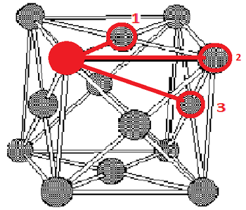
It is obvious from figure 3 that the lattice spacing in this lattice is just the difference between the atom under consideration and the atom labelled 2. Therefore, the lattice spacing must just be equal to the distance between the origin and the second nearest neighbour. The lattice spacing is equal to 1.525.

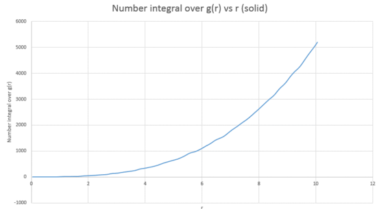
The coordination number of the atoms corresponding to the first three peaks of the FCC solid RDF can be calculated by comparing the number integral over $g(r)$ plot for the solid phase (graph 22) with the RDF plot for the solid (graph 23).

In graph 23, it can be seen that the first peak reaches a minimum at 1.275. If this figure for $r$ is read off the $\int g(r)\mathrm{d}r$ curve, then a value for the number integral can be obtained which corresponds to this peak; the coordination number for the first peak is therefore 12. This process is then repeated for the second peak, it reaches a minimum at 1.625 and the corresponding number integral over $g(r)$ is 18. If the coordination number of the first peak is then subtracted from 18 then the coordination for the second peak can be obtained; 6. If this is repeated once more, for a minumum in the RDF plot at 1.975 and corresponding number integral over $g(r)$ of 42. Subtraction then leaves a coordination number of 24 for peak three.

Graph 22 - Number integral over g(r)vs r (solid)

Graph 23 - RDF for the solid

Dynamical properties and the diffusion coefficient

This section will concentrate on the amount that the atoms in the system move around. This will be done by calculating the diffusion coefficient, $D$.

Mean squared displacement

$D$ can be calculated by using its connection to the mean squared displacement:

$D=\frac{1}{6}\frac{\partial ⟨r^2\left(t\right)⟩}{\partial t}$

It is a measure of the spatial extent of random motion. The mean squared value is taken to ensure that a positive value is obtained.

First, three simulations were run; on a solid, a liquid and a vapour. The temperature and density values from the previous section were used in the input files.

Graph 24 - Total mean squared displacement of the solid as a function of timestep

Graph 25 - Total mean squared displacement of the liquid as a function of timestep

Graph 26 - Total mean squared displacement of the vapour as a function of timestep

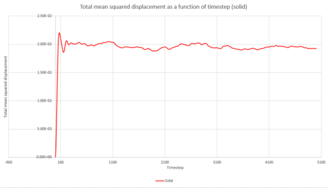
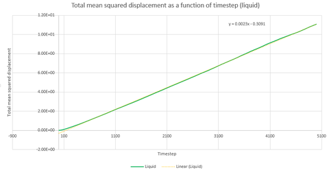
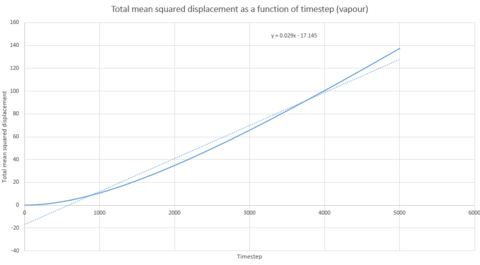
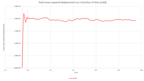
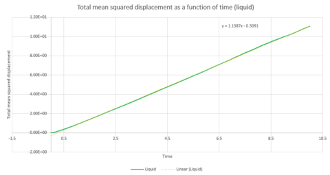
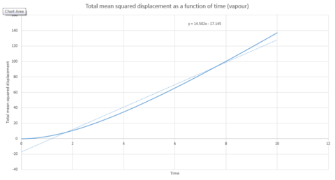
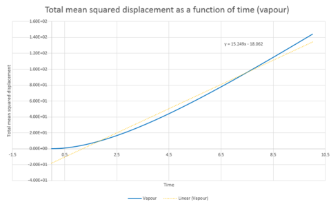
Graphs 24, 25 and 26 show the total mean squared displacement as a function of timestep for the three phases, solid, liquid and vapour respectively. It would be expected that the graphs would be of a linear fashion. This trend is followed for the plot of the liquid. However, the vapour plot can be seen to have a slight curve at the beginning. This is due to the lack of collisions at the start of the simulation in the low density vapour phase - the trend becomes linear after a collison. An atom in the high density solid is unable to move in a random fashion therefore the expected linear trend is not observed.

To calculate the diffusion coefficient, the x axis needs to be converted from units of timesteps to units of time. This can be seen in graphs 27, 28 and 29. The diffusion coefficient for these two graphs can therefore be calculated from the gradient of the data points. The gradient is multiplied by $\frac{1}{6}$ to obtain $D$.

Thus, if the graph for the liquid is considered first, the equation that resulted from the linear trendline was $y=1.1387x-0.3091$. The diffusion coefficient is therefore $1.387(\frac{1}{6})=0.190$ This process is also repeated for the solid and vapour phases.

Graph 27 - Total mean squared displacement of the solid as a function of time

Graph 28 - Total mean squared displacement of the liquid as a function of time

Graph 29 - Total mean squared displacement of the vapour as a function of time

The resulting gradients are shown in the below table:

	Solid	Liquid	Vapour
Gradient	3x10-6	1.1387	14.502
D	5x10-7	0.190	2.417

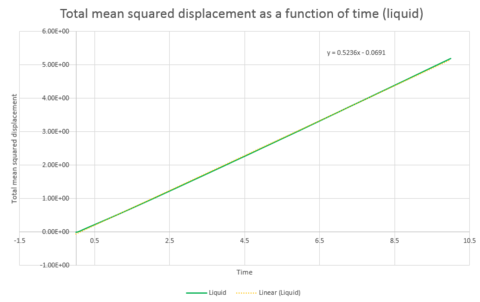
The above was repeated for a system of 1 million atoms. The total mean squared displacement as a function of time plots are shown in graphs 30, 31 and 32 and the resulting gradients and diffusion coefficients can be seen below.

	Solid	Liquid	Vapour
Gradient	3x10-5	0.5236	15.249
D	5x10-6	0.0873	2.54

Graph 30 - Total mean squared displacement of the solid as a function of time

Graph 31 - Total mean squared displacement of the liquid as a function of time

Graph 32 - Total mean squared displacement of the vapour as a function of time

The gradient of the plot for the solid was not taken over the entire graph, it was only taken over the section from graph 33.

Graph 33 - Total mean squared displacement of the solid as a function of time

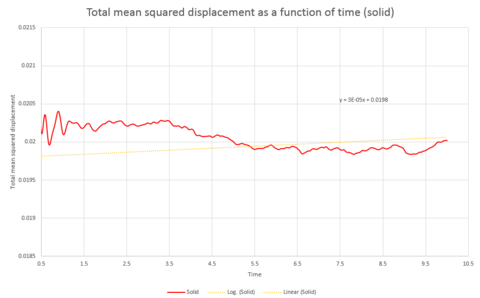
Comparison of the graphs of the systems of different sizes shows that the simulation with one million atoms provides smoother plots, this is to be expected for a larger system.

Velocity Autocorrelation Function

An alternative way of calculating the diffusion coefficient, $D$, is to use the velocity autocorrelation function which is given by the below equaiton:

$C\left(\tau \right)=⟨\mathbf{v}\left(t\right)\cdot \mathbf{v}(t+\tau )⟩$

This function states the difference in velocity at a time, $t+\tau$, compared with the starting time, $t$.

The equation for the evolution of the position of a 1D harmonic oscillator as a function of time;

$x\left(t\right)=A\cos (\omega t+\varphi )$

was used to evaluate the normalised velocity autocorrelation function for a 1D harmonic oscillator.

• because $x\left(t\right)=A\cos (\omega t+\varphi )$

• and we know that $v=\frac{dx}{dt}$

• the first equation can be differentiated to give

$v(\tau )=-A\omega \sin (\omega t+\varphi )$

• and therefore

$v(t+\tau )=-A\omega \sin (\omega (t+\tau )+\varphi )$

• If this is substituted into

$C\left(\tau \right)=\frac{\underset{-\mathrm{\infty }}{\overset{\mathrm{\infty }}{\int }}v\left(t\right)v(t+\tau )\mathrm{d}t}{\underset{-\mathrm{\infty }}{\overset{\mathrm{\infty }}{\int }}{v}^2\left(t\right)\mathrm{d}t}$

• Then this produces

$C\left(\tau \right)=\frac{\underset{-\mathrm{\infty }}{\overset{\mathrm{\infty }}{\int }}(-A\omega \sin (\omega t+\varphi ))(-A\omega \sin (\omega (t+\tau )+\varphi ))\mathrm{d}t}{\underset{-\mathrm{\infty }}{\overset{\mathrm{\infty }}{\int }}(-A\omega \sin (\omega t+\varphi ){)}^2\mathrm{d}t}$

• $C\left(\tau \right)=\frac{-A^2{\omega }^2\underset{-\mathrm{\infty }}{\overset{\mathrm{\infty }}{\int }}(\sin (\omega t+\varphi ))(\sin (\omega t+\omega \tau +\varphi ))\mathrm{d}t}{-A^2{\omega }^2\underset{-\mathrm{\infty }}{\overset{\mathrm{\infty }}{\int }}si{n}^2(\omega t+\varphi )\mathrm{d}t}$

• Because $\sin (\omega t+\varphi )+\omega \tau =\sin (\omega t+\varphi )\cos (\omega \tau )+\sin (\omega \tau )\cos (\omega t+\varphi )$

• The above therefore becomes

$C\left(\tau \right)=\frac{\underset{-\mathrm{\infty }}{\overset{\mathrm{\infty }}{\int }}[\sin (\omega t+\varphi )\cos (\omega \tau )+\sin (\omega \tau )\cos (\omega t+\varphi )][\sin (\omega t+\varphi )]\mathrm{d}t}{\underset{-\mathrm{\infty }}{\overset{\mathrm{\infty }}{\int }}si{n}^2(\omega t+\varphi )\mathrm{d}t}$

• $C\left(\tau \right)=\frac{\underset{-\mathrm{\infty }}{\overset{\mathrm{\infty }}{\int }}{\sin }^2(\omega t+\varphi )\cos (\omega \tau )+\sin (\omega \tau )\cos (\omega t+\varphi )\sin (\omega t+\varphi )\mathrm{d}t}{\underset{-\mathrm{\infty }}{\overset{\mathrm{\infty }}{\int }}si{n}^2(\omega t+\varphi )\mathrm{d}t}$

• $C\left(\tau \right)=\frac{\underset{-\mathrm{\infty }}{\overset{\mathrm{\infty }}{\int }}{\sin }^2(\omega t+\varphi )\cos (\omega \tau )\mathrm{d}t}{\underset{-\mathrm{\infty }}{\overset{\mathrm{\infty }}{\int }}si{n}^2(\omega t+\varphi )\mathrm{d}t}+\frac{\underset{-\mathrm{\infty }}{\overset{\mathrm{\infty }}{\int }}\sin (\omega \tau )\cos (\omega t+\varphi )\sin (\omega t+\varphi )\mathrm{d}t}{\underset{-\mathrm{\infty }}{\overset{\mathrm{\infty }}{\int }}si{n}^2(\omega t+\varphi )\mathrm{d}t}$

• The above will then cancel to

$C\left(\tau \right)=\cos (\omega \tau )+\frac{\underset{-\mathrm{\infty }}{\overset{\mathrm{\infty }}{\int }}\sin (\omega \tau )\cos (\omega t+\varphi )\sin (\omega t+\varphi )\mathrm{d}t}{\underset{-\mathrm{\infty }}{\overset{\mathrm{\infty }}{\int }}si{n}^2(\omega t+\varphi )\mathrm{d}t}$

• The function on the right hand side of the equation is odd. This means that when integrated, it will equal zero. Therefore, one final simplification can be made to produce:

$C\left(\tau \right)=\cos (\omega \tau )$

The final result of the above was then used, with $\omega =\frac{1}{2\pi }$, to plot the harmonic oscillator. This can be seen in graph 34. The VACFs for the liquid and the solid that were simulated above were also plotted on the same axis.

Graph 34 - VACF and harmonic oscillator as a function of time

The above procedure was then repeated for the system containing one million atoms, this can be seen in graph 35.

Graph 35 - VACF and harmonic oscillator as a function of time for 1 million particles

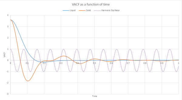
As can be seen from graphs 34 and 35, the VACF of the solid resembles the plot of the harmonic oscillator close to $\tau =0$ but then reaches a constant value with increasing time. The harmonic oscillator is such a consistent shape because it ignores all interactions with other particles and only experiences one single force while the particle under observation vibrates. The minima of the VACF plots represents the points where the particle changes its direction of velocity. In reality, the solid and the liquid both represent a damped harmonic oscillator because the attractive and repulsive forces they experience force the particles to settle to an equilibrium where the forces it is subjected to balance out, rather than continuously vibrating as in the harmonic oscillator. The solid suffers more oscillations than the liquid does. This is because the solid is more constricted than the liquid which means that the liquid isn't forced to oscillate as much because it is not fixed in a certain position.

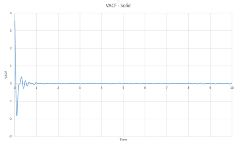
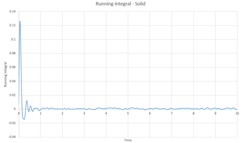
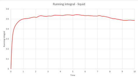
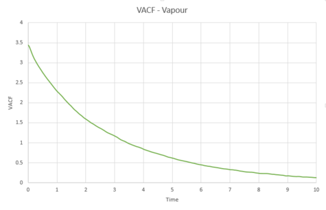
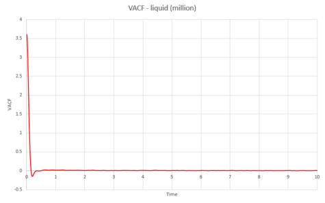
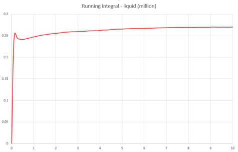
The trapezium rule was then used to approximate the integral under the velocity autocorrelation function for the solid, liquid, and gas. The graphs produced can be seen below as graphs 37, 39 and 41.

Graph 36 - VACF of solid

Graph 37 - Running integral - solid

Graph 38 - VACF of liquid

Graph 39 - Running integral - liquid

Graph 40 - VACF of vapour

Graph 41 - Running integral - vapour

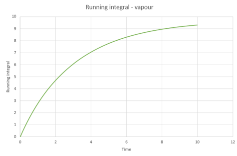The diffusion coefficients were calculated from these integrals, as shown below;

	Solid	Liquid	Vapour
D	1.44x10-4	0.181	3.11

It would be expected that the magnitude of the diffusion coefficients would follow the trend vapour > liquid > solid. This is because the atoms in the vapour are much further away from each other, meaning diffusion can take place with ease. Diffusion coefficient of the liquid would depend on its viscosity; a more viscous liquid would have a smaller $D$. The solid would be expected to have a very small value because very limited diffusion can take place in a solid. From the above table, this is true.

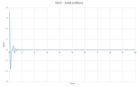
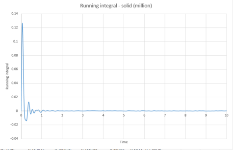
The above was then repeated for the simulated system of one million atoms.

Graph 42 - VACF of solid (one million)

Graph 43 - Running integral - solid (one million)

Graph 44 - VACF of liquid (one million)

Graph 45 - Running integral - liquid (one million)

Graph 46 - VACF of vapour (one million)

Graph 47 - Running integral - vapour (one million)

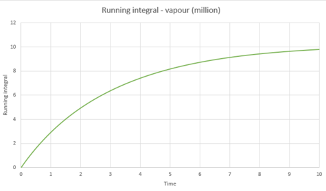The below diffusion coefficients were obtained for these systems from graphs 43, 45 and 47;

	Solid	Liquid	Vapour
D	1.22x10-4	0.089	3.26

These values for $D$ follow the same trend as explained above.

The largest source of error in the estimates of $D$ from the VACF would come from the use of the trapezium rule for the integration. The trapezium rule is an approximation which integrates the area under a curve by splitting up the area into multiple trapeziums and summing their individual areas. However, in this calculation, a very large number of trapeziums have been used and the accuracy increases with increasing number of trapeziums, meaning that this should be a good approximation to use in this case. This is shown to be true because similar values were calculated for the diffusion coefficients using the mean squared displacement and the velocity autocorrelation function.