
Rep:Jht114 Y3C MgO
Abstract
The General Utility Lattice Programe (GULP) was used to explore the variation of the Helmholtz Free Energy and thermal expansion of Magnesium Oxide with temperature. Using the Quasi-Harmonic Approximation (QHA), the phonon dispersion curve and phonon density of states (DOS) were computed. A grid size of 32x32x32 was found to be optimal to obtain convergence, and the variation of Free Energy with temperature is discussed. Also, the variation of the thermal expansion coefficient α with temperature was computed using the QHA and Molecular Dynamics. At low temperatures, α determined by the QHA is more accurate due to zero-point energy contributions; whereas at high temperatures, Molecular Dynamics gave a better representation of actual behaviour because QHA fails to account for bond breaking and phonon-phonon interactions. When the models did not break down (500 to 1100 K), α computed using both methods were about 20-30% smaller than experimentally determined values, which could be partly attributed to the simplification of the MgO lattice by neglecting ion polarizability.
Introduction
Vibrations in Solids
A multitude of properties, such as thermal expansion, heat capacity and transport properties, can be explored by studying vibrations in the solid state.[1] Thus, instead of static and completely rigid lattices, solids should be treated as dynamic structures with particles that are constantly fluctuating about their equilibrium positions. Since solids (crystals) are periodic arrays of particles (atoms, molecules or ions), the displacement of one particle will induce a displacement of neighbouring particles by exerting an attractive or repulsive force (Van der Waals, electrostatic etc), resulting in a periodic motion across the lattice.[2] This periodic displacement brought about by the vibration of particles can be described by oscillating harmonic waves. Similar to light waves, lattice vibrations can have particle-like properties, and analogous to photons, a quanta of lattice vibration is known as a phonon.

Considering first a simplified solid in 1 dimension (Figure 1), each vibrational mode has an associated wavelength and energy.
 (1)
(1)
where ħ is Planck's constant divided by 2π, n is the vibrational state, and ω is the frequency of the vibration, given by ω=2πc/λ.
The factor 0.5 ħω is from the contribution of the zero-point energy, i.e. the solid is never at rest. From Figure 1, it can be seen that the wavelength λ of the vibrations can range from 2a to infinity (corresponding to the in-phase motion of all atoms). Hence, even in 1-D, it is difficult to graphically depict and plot the vibrational modes in real space in terms of wavelength. Thus, the wave vector k is defined, where![]() . Analogous to photons, where momentum is given by
. Analogous to photons, where momentum is given by ![]() in the de Broglie equation, the wave vector k can be thought of as the momentum of phonons,
in the de Broglie equation, the wave vector k can be thought of as the momentum of phonons, ![]() . The introduction of the wave vector k enables all the vibrations to be represented in the k-space (reciprocal space), which has a range
. The introduction of the wave vector k enables all the vibrations to be represented in the k-space (reciprocal space), which has a range  (First Brillouin Zone). Any k-value outside the First Brillouin Zone (FBZ) would simply give a phonon already represented by within the FBZ due to the periodicity of the lattice.
The relationship between the wave vector k and frequency ω is known as phonon dispersion. In a 1-dimensional monoatomic solid, the dependence of ω on k is given by:
 (2) [3]
where J is the force constant, a is the lattice separation, and M is mass of the particle. In comparison, for a 1-dimensional diatomic solid, the relationship is given by:
 (3)[3]
Thus, two possible ωk values for each k can be obtained for a diatomic solid. To generalize, the number of frequencies ω (degrees of freedom) obtained at each k is proportional to the number of particles (N) in the unit cell, i.e. 1N for a one-dimensional structure of N particles.
Applying this to a 3-dimensional solid, each atom in the solid can oscillate in 3 different directions. Hence, the degrees of freedom and number of branches is 3N. Rotation is not possible in the solid, and translation is the in-phase motion of all atoms, which is accounted for in the acoustic band. As such, there is no 3N-5/6 as compared to gaseous particles. Thus, for the MgO primitive cell, which has 2 atoms, 6 branches are expected.
Dispersion curves
To represent the vibrations in the reciprocal space, a dispersion curve is used. The frequency ω is plotted against k. Figure 2 is an example of a dispersion curve for a 1-dimensional diatomic solid.

The acoustic mode is where the atoms in the unit cell vibrate in-phase, whereas the optic modes is where the atoms in the unit cell vibrate out-of-phase. At k = ±π/a, the motions of adjacent unit cells are opposite to each other, and the lattice has zero group velocity, giving dω/dk=0. Experimentally, the dispersion curves can be determined via inelastic neutron scattering. [4]
Density of States (DOS)
Thermodynamic properties depend directly on frequency of normal mode ω, not the wave vector k.[3] Hence, to obtain all the normal mode frequencies, grids can be generated in the reciprocal space to collect a sample of frequency values. If the grids are sufficiently fine to represent all the vibrational modes, a histogram of frequencies is obtained, which is known as the density of states.
This then allows for thermodynamic properties to be represented as an integral. For example, total vibrational energy E:
 (4)[3]
where g(ω) is the density of states.
Quasi-Harmonic Approximation (QHA)
Whilst the potential between atoms are anharmonic, the Harmonic Approximation is still a key approximation in Lattice Dynamics.[5] In this approximation, the Taylor's expansion for the energy is retained until the quadratic term.[3,5] The Harmonic Approximation (HA) is powerful because it enables the link between vibrational frequency, interatomic forces, wave vectors, and other thermodynamic properties to be established. However, volume-dependent properties such as thermal expansion, thermal conductivity and phase transitions cannot be determined from this approximation. Thus, the Harmonic Approximation is usually used as a starting point, with additional terms or parameters being introduced subsequently to capture anharmonicity.[3]
In this simulation, the Quasi-Harmonic Approximation (QHA) is used. In the QHA, the harmonic potential is retained, but the frequency of phonons are allowed to vary with volume. Thus, this approximation does not capture the full anharmonicity of the system. Nonetheless, it still allows volume-dependent properties, such as thermal expansion, to be determined.

From Figure 3, it can be seen that the QHA does not fully capture the anharmonicity of a system. One of the limitations of the QHA is that it does not allow for bond breaking - in Figure 3, the QHA potential energy curve increases to infinity as the bond lengthens, rather than to a constant value in the anharmonic curve. Also, the QHA does not account for phonon-phonon interactions. The combination of these limitations render this approximation accurate only up to 50-70% of the melting temperature.[6]
Molecular Dynamics (MD)
The Molecular Dynamics simulation predicts properties of assemblies by numerically solving classical Newtonian equations:[7]
 (5,6)
(5,6)
where r is distance between particles, F is the force acting on a particle and U is potential energy between the particles. The potential energy U can be quantified by different models, such as Hooke's Law potential,[7] or pair-potentials (Leonard Jones potential, Buckingham potential).[8]
Essentially, the MgO lattice has an associated energy when the atoms are at specific positions. In the molecular dynamics method, each MgO primitive cell is treated as a molecule. Then, from the equipartition theory,
 (7)
(7)
a random speed is assigned to each molecule (MgO) based on temperature. Based on the Verlet algorithm,[7] the following sequence of calculations are carried out:
1. Based on speed v0, a new position is calculated based on timestep δt:  r1 = r0 + v0 • δt
2. When moved to the new position r1, the particles experience a new force F due to electrostatic and repulsive interactions
3. The acceleration a of particle is calculated by a=F/m
4. Then the new velocity is calculated by: v1 = v0 + a • δt
5. New positions are then computed based on this velocity.
6. These calculations are repeated until the energy and atomic position settles down.
In contrast to the Quasi-Harmonic Approximation, Molecular Dynamics operates in real space. Hence, the size of the cell used is important in determining the vibrational modes that can be represented. In the reciprocal space, the primitive cell is sufficient to represent all vibrational modes. However, in the real space, a larger cell entails a more accurate representation of the possible vibrational modes due to the larger number of modes that can be explored. Thus, in order to determine the optimum cell size considering accuracy and computational cost, a convergence test can be used. This involves increasing the cell size used in each simulation, until the difference in the results obtained is within the desired accuracy. Another point to note on the efficiency of the calculation is the timestep. Whilst a smaller timestep gives a better numerical stability, doing so incurs a higher computational cost.
The limitations of the MD simulation differs from that of the QHA simulation, since it involves classical mechanics instead of quantum mechanics used in the QHA. Thus, the MD simulation fails at low temperatures, where quantum mechanical effects become more prominent.[9] This could be understood in terms of the zero-point energy, which states that particles are not at rest even at 0 K, in contrast to that predicted in classical mechanics.
MgO Structure
MgO is of importance in various fields such as solid-state physics and earth-science, due to its high refractoriness, thermal conductivity, and natural abundance.[10] Thus, the thermodynamic and bulk properties of MgO are of interest.
The periodic MgO lattice can be described using different unit cells. The primitive cell can be used, which consists of 1 Mg and 1 O atom in a rhombohedron with an internal angle of 60°. Alternatively, the conventional cell, which better captures the cubic symmetric of the lattice, consists of 4 Mg and 4 O atoms in a face-centered cubic (FCC) system can also be used. Since MgO is a cubic system, only one lattice parameter is required to describe the cell, which is the length of the edge of the conventional cell. Both cells are depicted in Figure 4 below.

The conventional cell has 4 times the number of atoms of a primitive cell, so Mc=4Mp. Since both the cells are from the same material and lattice, they have equal densities ρc=ρp. Since ρ=M/V, Vc=4Vp. From this, it is possible to convert between the lattice parameters of different cells
Thermal Expansion
Thermal expansion is the increase in volume of a material brought about by an increase in temperature. In the Harmonic Approximation, thermal expansion is not possible since the equilibrium separation remains the same regardless of the excited state (Figure 3, grey dotted line). In contrast, in an anharmonic system, excited states have longer equilibrium separations. (Figure 3, blue dots). By increasing the temperature, more excited states are populated, and hence the average separation of atoms in the lattice increases. This is the physical reason for thermal expansion. The thermal expansion coefficient α, which gives the quantifies the increase in volume with respect to temperature, can then be calculated by Equation 8:
 (8)
(8)
Methodology
All simulations were carried out using GULP in the Linux environment.
Quasi-Harmonic Approximation
The pressure was set to 0 GPa in all simulations.
The Buckingham potential (Eqn 9) was used to quantify the short-range interaction between Mg2+ and O2- ions.[11] The ionic shells were not included, such that the ions are treated as unpolarizable hard spheres. This would be a reasonable approximation, given that both Mg2+ and O2-, filled up to the 2p shell, are 'hard' ions with low polarizability.
 (9)[12]
Where A, B and C are constants related to the type of lattice. In this calculation, the MgO primitive cell with the following parameters was used in the calculation:
Cell vectors (Å): 0.0000   2.10597   2.10597
                  2.10597   0.0000   2.10597
                  2.10597   2.10597   0.0000
ap (Å)          : 2.9783
Phonon Dispersion Curve
Each vibrational mode (phonon) of the MgO primitive cell has an associated wavevector k. In this simulation, the phonons of 50 k-values along the conventional path in the k-space (W-L-G-W-X-K) were computed at 300 K, yielding a phonon dispersion curve.
At each k-value, 6 vibrations are obtained, corresponding to the 3N number of branches (N=2) in the primitive cell.
Density of States
Ideally, the density of states (DOS) is computed by an analytical integration across the frequencies obtained in the First Brillouin Zone. However, this is not possible, so numerical methods must be employed. To achieve this, the First Brillouin Zone is divided into grids specified by the shrinking factor,[13] which determines the number of samplings from the dispersion curve used to compute the DOS curve. The phonon frequencies at the specified k-values are computed, and the occurrence of each photon frequency is collated and normalized to yield the density of states. The larger the shrinking factor (grid size), the more accurate the approximation of the analytical solution is obtained, at the cost of computational power. The shrinking factors (along each kx,y,z direction) used in this simulation were 1x1x1, 2x2x2, 4x4x4, 8x8x8, 16x16x16, 32x32x32 and 64x64x64.
Helmholtz Free Energy
Statistical thermodynamics was employed to obtain the thermodynamic properties from the microscopic properties computed in the Quasi-Harmonic Approximation. This can be done by the summation across all the vibrational modes in Equations 10 and 11 below.
Under the Harmonic Approximation, the Helmholtz Free Energy F is given by:
 (10)[3]
where E0 is the Lattice energy, ωk,j is the vibrational frequency with wavevector k in the j-th band, and kB is the Boltzmann constant. The first two terms in the equation arise from the contribution of the Internal Energy U of the system, whereas the third term is the entropic contribution. In this experiment the Quasi-Harmonic Approximation was employed, where an explicit volume dependence (V) was introduced for the frequencies:
 (11)[3]
The Helmholtz Free Energy was computed at T=300 K, and grid sizes of 1x1x1, 2x2x2, 4x4x4, 8x8x8, 16x16x16, 32x32x32 and 64x64x64 were used to test for convergence. Since the 32x32x32 grid was determined to be the optimal grid size, it was used to compute the Helmholtz Free Energy from 0 to 3000 K.
Thermal Expansion of MgO
Since the Helmholtz Energy describes a system at constant volume, it does not allow for the minimisation of free energy with respect to volume change. Thus, the equilibrium volume V(P,T) was determined by minimising Gibbs Free Energy G. From Equation (11), a Legendre Transform could be performed on the Helmholtz Energy F(N,V,T) to obtain a new free energy function dependent of a new set of thermodynamic variables G(N,P,T). The equilibrium volume was then computed from 0 to 3000 K, slightly below the melting point of MgO. (3098 K)[14] A grid size of 32x32x32 was used since this was the smallest grid size that gave convergence for the Helmholtz Free Energy calculation. From the equilibrium volumes, the thermal expansion coefficient was then computed using Equation (8).
Molecular Dynamics
The following parameters were used to compute the properties of a supercell made up of 32 MgO primitive cells:
Ensemble           : NPT
Timestep δt        : 1 fs
Temperature        : 0 to 3000 K
Equilibration steps: 500
Production steps   : 500
Sampling steps     : 5
Trajectory steps   : 5
The equlibrium volumes were obtained and used to calculate the thermal expansion coefficient.
Results and Discussion
Phonon modes of MgO
The phonon dispersion curve and DOS plots obtained are presented below. The DOS for the shrinking factor 32x32x32 is compared to the dispersion curve.

|
 |
| Figure 5: Phonon Dispersion Curve obtained for 50 points along the conventional path, compared to the DOS plot obtained using a shrinking factor of 32x32x32. | |

It can be seen that the dispersion curve calculated in this simulation (Figure 5) shows reasonable agreement with that of the literature (Figure 6) in terms of the general band structure. However, it can be noted that the DOS calculated in this simulation showed 3 peaks merging around 400 cm-1, whereas the literature data (Figure 6) showed 3 distinct peaks separated at 280, 450 and 550 cm-1. One reason for this lack of accuracy in this simulation could be the exclusion of long-range forces, which was accounted for in the work of Artem et al. via density-functional pertubation theory.
Nonetheless, the dispersion curve in Figure 5 can still be analysed qualitatively. In Figure 5, each k-value gives 6 frequencies, resulting in 6 branches. This is expected since a 3-dimensional system of 2 atoms was considered. However, some of the frequencies are degenerate, resulting in lesser than 6 frequencies observed at certain k-values. Also, it can be seen that the density of states is highest where the dispersion curve has a flat shape, since these would correspond to the largest number of phonons.
The DOS curves for the different grid sizes are presented below.

|

|

|
| Figure 8: DOS curve for shrinking factor of 2x2x2 | Figure 9: DOS curve for shrinking factor of 4x4x4 | Figure 10: DOS curve for shrinking factor of 8x8x8 |

|

|

|
| Figure 11: DOS curve for shrinking factor of 16x16x16 | Figure 12: DOS curve for shrinking factor of 32x32x32 | Figure 13: DOS curve for shrinking factor of 64x64x64 |
First, it should be noted that the number of samplings collected to obtain the DOS plot is smaller than number of grids used. This is due to cubic symmetry of the k-space across the [200] plane, resulting in the phonon frequencies computed along both halves to be the same. Thus, the number of samplings conducted was exactly half the number of grids, and can be thought of as cutting a cube in half along the [200] plane, and only sampling the frequencies of the k-values in one half, saving computational cost.
Initially, as grid size increases, more peaks appear on the DOS curves since more frequencies are being sampled. As the grid size increases further, the DOS plots becomes smoother since the number of k-points sampled increases. The shrinking factor of 32x32x32 gave a reasonably similar curve as compared to that of 64x64x64, indicating convergence. The 32x32x32 grid took considerably less time, hence lower computational cost. Thus, for the primitive MgO cell, 32x32x32 is the optimum grid size that gives a reasonable accuracy without incurring a large computational cost.
The number of grids required to achieve the same accuracy depends on the type of unit cell used (e.g. primitive/conventional/supercell), even for the same compound. For MgO, if the conventional cell is used, the k-space will be smaller than that of this experiment. This is because
 (12)
(12)
For the conventional cell, a = 4.212 Å, whereas for the primitive cell, a = 2.9783 Å.[15] Thus, a* for the conventional MgO cell is smaller, and it has a smaller k-space. Hence, a smaller number of grids is sufficient to achieve same accuracy as that of the primitive cell. For each k-point, a larger number of vibrations are being sampled (24 for a conventional cell vs 6 in primitive cell), by virtue of the unit cell having more atoms. This would then result in more bands, where the conventional cell would have 24 bands due to 8 atoms in 3 dimensions. The band structure of the conventional cell can be predicted from the band structure of the primitive cell by the 'folding process' described by Hoffmann.[16]
In the following discussion for the optimum grid size required for CaO, Zeolite and Lithium, to keep the symmetry of the unit cell the same as MgO, the comparison is being done on the conventional cell, where all have cubic symmetries. Zeolite (Faujasite) has a = 24.34 Å,[17] which is much larger than that of MgO. Thus, the k-space is much smaller, and a smaller grid is sufficient to achieve the same accuracy. For a similar metal oxide (CaO), a = 4.81 Å,[18] which is similar in magnitude to that of MgO, the grid required would be similar to that of MgO. Lastly, Li has a = 3.51 Å,[19] which is smaller than that of MgO. Thus, a larger grid is expected to be required to achieve the same accuracy when compared to MgO.
Free Energy vs Grid Size
The calculation of Free energy with respect to grid size is shown in Figure 14 below:

From Figure 14, the Free Energy converges to a value of -40.926483 eV. When a small gird is used, the convergence is poor due to the small number of frequencies sampled, so there is a large difference in Free Energy as the grid is increased initially. However, as the number of grids used is further increased, the convergence improves, hence resulting in a smaller difference in the newly computed value and the grid size used previously. (Table 1) Specifically, the Free Energy converges to a reasonable estimate after the 8x8x8 grid.
A summary of the difference in the in the Free Energy with respect to the previous grid size is presented in Table 1:
| Table 1: Difference in computed free energies compared to the previous grid size. | |
|---|---|
| Grid Size (MxMxM) | ΔF (FM-FM/2) / meV |
| 1x1x1 | n/a |
| 2x2x2 | 3.692 |
| 4x4x4 | 0.159 |
| 8x8x8 | -0.028 |
| 16x16x16 | -0.004 |
| 32x32x32 | -0.001 |
| 64x64x64 | 0 |
Thus, a grid size of 4x4x4 was sufficient for calculations accurate to 1 and 0.5 meV, whereas a 8x8x8 grid size is sufficient for that up to 0.1 eV. To achieve convergence at the lowest compuational cost, a 32x32x32 grid was sufficient. However, further optimisation could be done by decreasing the grid to 31x31x31, and further downwards to investigate the convergence at lower computational costs.
Free Energy vs Temperature (Lattice Dynamics)
The variation of Helmholtz Free Energy A with temperature is shown in Figure 15:

From A = U - TS, the free energy is expected to decrease linearly as temperature increases. However, this is not the case since the entropic term is temperature dependent, as described in Equation 11. At low temperatures, the temperature dependence of the free energy is small. This is because in the third term in Equation 11, as T approaches 0, the following relationship holds:
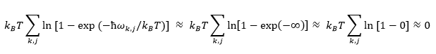

Since ln 1 = 0, the linear dependence of A on temperature (TS term) disappears, and the Free Energy Equation (11) reduces to the first two terms, which are temperature independent. Thus, curve approaches that of a horizontal line. At 'medium' temperatures, the entropic contribution now becomes significant, and there is a linear dependence on temperature.
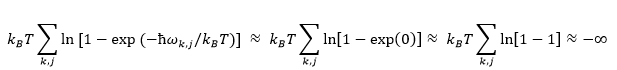
As the temperature becomes 'high', the free energy decreases exponentially. This is due to the anharmonicity of the potential well, where the energy spacing (Δћω) decreases towards the top of the well, due to the decrease in frequency ω of phonons when volume increases. The decrease in frequency of photons as volume increases is due to the increase in equilibrium separation a, which results in an increase in wavelength. Since wavelength is inversely related to frequency, when wavelength increases, the frequency decreases. The result of this is that excited states become more easily populated as temperature increases, resulting in a large increase in entropy. Hence, the entropic contribution is no longer linear, and A shows a larger than expected decrease as T approaches infinity because of the following:

Lattice Parameter vs Temperature
The variation of the lattice parameter a with temperature is shown in Figure 16.

At low temperatures (between 0 to 400 K), the lattice parameter does not increase linearly, and there is a very small increase in size. This is due to the contribution from the zero-point energy, which causes the atoms to vibrate even at 0 K. These vibrations result in solids occupying a larger volume than expected in classical mechanics. At low temperatures, only the ground state vibration is populated, and thus there is no significant increase in volume. At high temperatures (1500 K), similar to the Helmholtz Free Energy, excited vibrational states are more easily populated due to a smaller Δħω. Hence, the atoms spend more time in states with larger equilibrium positions, and the increase in lattice parameter is larger than expected. This result highlights one of the failures of the Quasi-Harmonic Approximation, where the volume is allowed to expand infinitely without taking into account bond breaking and phonon-phonon interactions at high temperatures. Essentially, near the melting temperature, the system should no longer be treated as a periodic lattice with quantized vibrational modes as was done in this simulation. Rather, it behaves as a liquid-like material where particles have more translational freedom.
Thermal Expansion of MgO
The thermal expansion coefficient α is an intensive property, since it is being normalized by dividing by V0. (Equation 8) Thus, the expansion coefficient should be the same regardless of the lattice size investigated, and can be compared across the MD and LD methods. In this report, V is taken to be the volume of the primitive cell. First, the variation in V with T is being shown in Figure 17:

The shape of the curve obtained by lattice dynamics (LD) could be explained using the same arguments as that in the section above, since the increase in lattice parameter a is analogous to the increase in volume. In the Molecular Dynamics approximation, the increase in volume is proportional to temperature. The plot was fitted to a polynomial of order 6 to obtain a higher accuracy for the calculation of the thermal expansion coefficient. However, fitting a linear equation gave R2 = 0.9941, which is reasonably high to conclude that in this method, the increase in volume has a linear relationship to temperature. This is expected, since Molecular Dynamics solves classical Newtonian equations to predict the properties of a system. Thus, even at high temperatures, a linear increase in volume is expected, as contrast to the infinite increase as predicted in the QHA.
Both the Quasi-Harmonic Approximation (Lattice Dynamics) and Molecular Dynamics gave different results. This is due to the different systems of equations that are being solved. The QHA uses a quantum mechanical approach that solves for the equilibrium position of the atoms by minimising the free energy. Then, statistical thermodynamics is used to solve for macroscopic parameters. In contrast, MD uses classical mechanics to solve for molecular separation by allowing the total energy of the system to reach an equilibrium. Since both methods adopt fundamentally different approaches, they are expected to give different results.
Expansion Coefficient vs Temperature
From the fitted equations in Figure 17, the gradient at each point was calculated by differentiation. This was then used to obtain the expansion coefficient α by dividing with V0, (Equation 8) which is the initial volume of the cell for each calculation.
| Calculated (this experiment) | Literature |
|---|---|
 |
 |
| Figure 18: Comparing shapes of curves of computational inputs to Figure 19 (beside), the data obtained from LD has a similar shape to that of computed literature values, whereas the data obtained using MD seemingly fluctuates around a linear line. Experimental data was obtained from the work of Anderson et al.[20] | Figure 19: Literature data obtained by A. Erba et al[1]
by computational methods (DFT, QHA) using CRYSTAL-14, and that obtained by Anderson et al and Ganesan et al by experimental measurements. |
Data from experimental sources showed a linear increase from 1000 to 3000 K. Hence, both quantum mechanical computational models (this experiment and that used by Erba et al) breaks down at high T. (above 1700 K for this simulation, above 1100 K for A. Erba et al.) This is because of long range phonon-phonon interactions, and also because the QHA doesn't allow for bond breaking. In contrast, for this temperature range, the molecular dynamics method works (somewhat) better in terms of predicting the general linear increasing trend of the thermal expansion at high temperatures. This could be attributed to the fact that Molecular Dynamics does not require the ions to be positioned on fixed lattice points, but are instead allowed to move and translate freely to obtain the equilibrium geometry of lowest energy. In this case, below the melting point, the equilibrium geometry has a periodic arrangement which coincides with that of a solid structure. Thus, near the melting point, the type of motions explored in MD better simulates the actual behaviour of solids, and gives a more accurate prediction of the bulk properties.
However, the the thermal expansion coefficients computed using Molecular Dynamics have a seemingly large fluctuation about the linear fit. One possible reason for this noisiness could be attributed to the small size of the supercell used, which only contained 32 MgO Units (64 atoms), and is insufficient to account for all the possible vibrational modes in bulk MgO. To determine the size of the supercell that should be used, parallels could be drawn to optimisation of grid size used in the QHA method. In other words, the size of the unit cell used in the MD simulation could be increased until convergence is obtained. Through this, less fluctuations would be observed, and a more accurate estimate could be obtained.
At low T (0 to 500 K), however, the Quasi-Harmonic Approximation works better than Molecular Dynamics since it takes into account zero point energy, which is a quantum mechanical property that is not accounted for in classical mechanics. For this reason, the MD simulation failed to work at 0 K, since there is no motion at 0 K in classical mechanics. Also, at low T, Molecular Dynamics overestimates thermal expansion, since it predicts a linear increase in volume, when in fact, the population of the ground vibrational state means that the increase in volume is insignificant at low T.
It should be noted that, in contrast to literature computed values, the thermal expansion coefficients computed in this experiment (both QHA and MD) did not converge with experimentally obtained values. Although the same order of magnitude is obtained, the values computed in this experiment are about 25% smaller than experimentally determined values. This could be attributed to the various parameters not considered in the calculation, such as the shells of the Mg2+ and O2- ions, which gives rise to the polarisability of the ions, or the inclusion of ionic potentials in the Buckingham potential equation.
Phyiscal basis for thermal expansion in LD vs MD
Although both models correctly predict for the increase in volume with temperature, the physical basis for this expansion is different for both. In lattice dynamics, the explanation is described in the introduction section, where the population of excited states with larger equilibrium separations in the anharmonic potential well results in volume expansion. In molecular dynamics, this is due to the dependence of the kinetic and potential energies of the system on temperature.[21] At higher temperatures, the equilibrium separation of the particles in the solid lattice is increased in order to minimise the total energy of the system. Thus, this forms the basis for thermal expansion in molecular dynamics.
Conclusions
Using the Quasi-Harmonic Approximation, the phonon dispersion curve was obtained using GULP. 6 branches were obtained, as expected for a 2-atom primitive MgO cell. The density of states were obtained using grid sizes of 1x1x1 up to 64x64x64, where convergences was obtained at the 32x32x32 grid size. The shapes of the curve are generally in agreement with experimentally determined curves, but with some inconsistencies.
Similarly, a grid size of 32x32x32 was sufficient for convergence to be obtained for the Helmholtz Free Energy, which was found to decrease with temperature. At low temperatures, the decrease was small due to low entropic contribution. The decrease was then found to be exponential at higher temperatures due to the large increase in entropic contribution, which leads to the inference that entropy is temperature-dependent.
When the thermal expansion was examined via the QHA, there was a small increase in volume V at low temperature. This is due to population of the ground vibrational state as kBT<<Δħω. The increase in volume then became linear, and at high T there was a quadratic increase. When examined using Molecular Dynamics, the volume increased linearly at all temperatures.
In essence, at low and high temperatures, there was a large variation in thermal expansion coefficients predicted by both methods. At low T, the QHA was more accurate, and MD overestimates α because it neglects zero-point energy contributions. At high T, MD is more accurate, and QHA overestimates α due to bond breaking and phonon-phonon interactions. Both methods converge at 500-1100 K.
Lastly, even though for the properties examined using the QHA converged internally, insufficient parameters were used to model actual behaviour of ions (e.g. polarizability). For MD, the cell size used was too small to accurately represent all possible vibrational modes. As a result, α computed in both methods were 20-30% lower than experimental values.
Further work
One possible aspect where further work could be done is to determine the optimal grid size in the QHA. In this computation, grid sizes were varied in increments of 2x. Thus, a smaller variation could be examined below the converged grid size (32x32x32) obtained. For instance, 30x30x30 could be examined if it could be used to obtain convergence at a lower computational cost.
Next, more parameters could be introduced to model the system. For instance, the Buckingham potential could be modified to include Coulombic interactions, described by the Coulomb-Buckingham potential:[22]

Also, polarizability of the ions could be introduced via density functional theory. However, the inclusion of these parameters would incur significantly higher computational costs and requires modification of the current algorithms.
References
- ↑ A. Erba, M. Shahrokhi, R. Moradian and R. Dovesi, J. Chem. Phys., 2015, 142, 44114.
- ↑ M. T. Dove, Collect. SFN, 2011, 12, 123–159
- ↑ P. K. Misra, in Physics of Condensed Matter, Academic Press, 2012, pp. 37–47.
- ↑ G. Peckham, Proc. Phys. Soc., 1967, 90, 657–670.
- ↑ A. A. Maradudin, E. W. Montrol and G. H. Weiss, in Theory of Lattice Dynamics in the Harmonic Approximation, Academic Pess, 1963, pp. 5–29.
- ↑ J. M. Skelton, D. Tiana, S. C. Parker, A. Togo, I. Tanaka and A. Walsh, J. Chem. Phys., 2015, 143, 64710.
- ↑ V. E. Lamberti, L. D. Fosdick, E. R. Jessup and C. J. C. Schauble, J. Chem. Educ., 2002, 79, 601.
- ↑ M. P. Allen, Comput. Soft Matter, 2004, 23, 1–28.
- ↑ J. Meller, Encycl. Life Sci., 2001, 1–8
- ↑ A. R. Oganov, M. J. Gillan and G. D. Price, J. Chem. Phys., 2003, 118, 10174–10182.
- ↑ T. S. Bush, J. D. Gale, C. R. A. Catlow and P. D. Battle, J. Mater. Chem., 1994, 4, 831.
- ↑ V. Migliorati, A. Serva, F. M. Terenzio and P. D’Angelo, Inorg. Chem., 2017, 56, 6214–6224.
- ↑ R. Ramirez and M. C. Böhm, Int. J. Quantum Chem., 1988, 34, 571–594.
- ↑ W. M. Haynes, in CRC Handbook of Chemistry and Physics : a ready-reference book of chemical and physical data, CRC Press, 92nd edn., 2011, pp. 4–74.
- ↑ C. A. and editors of the volumes III/17B-22A-41B, in II-VI and I-VII Compounds; Semimagnetic Compounds, Springer-Verlag, Berlin/Heidelberg, pp. 1–6.
- ↑ R. Hoffmann, Angew. Chemie Int. Ed. English, 1987, 26, 846–878.
- ↑ E. L. First, C. E. Gounaris, J. Wei and C. A. Floudas, Phys. Chem. Chem. Phys., 2011, 13, 17339.
- ↑ C. H. Shen, R. S. Liu, J. G. Lin and C. Y. Huang, Mater. Res. Bull., 2001, 36, 1139–1148.
- ↑ M. R. Nadler and C. P. Kempier, Anal. Chem., 1959, 31, 2109–2109.
- ↑ O. L. Anderson, D. Isaak and H. Oda, Rev. Geophys., 1992, 30, 57.
- ↑ V. Timon, S. Brand, S. J. Clark and R. A. Abram, J. Phys. Condens. Matter, 2006, 18, 3489–3498.
- ↑ K. P. Chong, A. P. Boresi, S. Saigal and J. D. Lee, in Numerical Methods in Mechanics of Materials : with Applications from nano to macro scales, CRC Press, 2017, p. 229