Introduction to the Ising Model

The Model

Minimum Energy State

Minimum Interaction Energy

The interaction energy of an Ising lattice is given by:

$E = - \frac{1}{2} J \sum_{i}^{N} \sum_{j \in n e i g h b o u r s (i)} s_{i} s_{j}$

In an Ising lattice with D dimensions and periodic boundary conditions, a given spin $s_{i}$ has 2D neighbours.

The minimum interaction energy is achieved when all spins in the lattice are aligned (all ↑ or all ↓). As such, any spin $s_{i}$ must be aligned with all 2D of its neighbours. That is, $s_{i} s_{j} = 1$ for all $j$ .

Therefore, for any $s_{i}$ , the sum of its interactions is $\sum_{j \in n e i g h b o u r s (i)} s_{i} s_{j} = 2 D$

As this is true for all N spins in the lattice, it follows that $\sum_{i}^{N} 2 D = 2 D N$ .

Thus the minimum interaction energy is given by:

E_{m i n} = - \frac{1}{2} J \cdot 2 D N = - D N J

Entropy of the Minimum Energy State

The entropy of a state is given by:

S = k l n Ω

Where $Ω$ is the multiplicity of the state, the number of degenerate configurations of said state. The minimum energy state is achievable with all spins ↑ or with all spins ↓. In the absence of an external magnetic field, these configurations are degenerate and indistinguishable giving $Ω = 2$ for this state. Therefore,

$S_{E_{m i n}} = k_{B} l n 2 = 0.693 k_{B} = 9.57 \times 1 0^{- 24} J \cdot K^{- 1}$

Phase Transitions

Changes to Minimum Energy Configuration

Energy Change

The energy change $Δ E$ associated with a single spin 'flip' from the lowest energy onfiguration may be calculated by considering the change in the interaction energy with the spin's neighbours.

Let $D = 3, N = 1000$

$Δ E = E_{1} - E_{0}$

$E_{1}$ Interaction energy after one spin has been 'flipped'

$E_{0}$ Lowest energy configuration

$\sum_{i n t e r a c t i o n s} = - 2 D + 2 D (2 D - 2) + 2 D [N - (2 D + 1)]$

$= 2 D N - 8 D$

$E_{1} = - \frac{1}{2} J \sum_{i n t e r a c t i o n s} = 4 D J - D N J$

$Δ E = E_{1} - E_{0} = 4 D J - D N J + D N J = + 4 D J = + 12 J$

This energy change is independent of $N$ and depends only on the dimension size and the coupling constant $J$ .

In this calculation, the following assumption has been made.

The lattice dimensions are infinite relative to the size of each cell

This allows any cell to be treated as the centre of the lattice. As every cell interacts with 2D neighbours, flipping any cell in the minimum energy configuration results in the same energy change. Alternatively, the periodic boundary conditions of the Ising model remove the necessity for such an assumption. As a consequence, the absence of $N$ from the resulting energy change is justified.

Entropy Change

$S = k_{B} l n Ω$

$Ω = \frac{N!}{N_{↑}! N_{↓}!}$

Where $N_{x}!$ denotes the factorial of the number of spins in spin state $x$ .

$Δ S = k_{B} l n (\frac{Ω_{2}}{Ω_{1}})$

$Ω_{2} = \frac{1000!}{999! 1!} = 1000$

$Ω_{1} = \frac{1000!}{1000!} = 1$

$Δ S = k_{B} l n 1000 = 9.54 \times 1 0^{- 23} J K^{- 1}$

$Δ S_{m o l} = N_{A} k_{B} l n 1000 = 57.4 J K^{- 1} m o l^{- 1}$

Magnetisation Values of 1D and 2D Lattices

$M = \sum_{i} s_{i}$

1D Lattice Magnetisation

$M_{1 D} = + 1$

2D Lattice Magnetisation

$M_{2 D} = + 1$

Magnetisation at 0K

At 0K, no thermal energy is available to overcome the energetic barriers to spin flipping. Considering the Hemholtz free energy:

$A = E - T S$

A temperature of 0K nullifies the entropic contribution to the free energy. Thus the energetic driving force (which maximises parallel spin interactions) dominates the entropic driving force (which maximises multiplicity of lattice states). For an Ising Lattice with D = 3, N = 1000 at 0K, the alignment of all spins results in the minimum energy configuration and an overall magnetisation of $M = \pm 1000$ .

Calculating the Energy and Magnetisation

Modifying the Files

Energy and Magnetisation Functions

=Energy

The above energy method segments a given lattice into lattice cells on the edges, corners or in the bulk of the lattice and calculates the energy interactions with its neighbours as appropriate.

Magnetisation

The magnetisation method loops over all elements in the array representing the Ising lattice and adds the value of the spin to the magnetisation variable.

Testing the Files

ILCheck.py

Above, the results of the ILcheck.py script are presented.

Introduction to the Monte Carlo Simulation

Average Energy and Magnetisation

Configurations of a 100 Spin System

For a system of two spins, 4 configurations are possible (↑↑, ↓↓, ↑↓, ↓↑) i.e. $2^{2}$ . For a system of 100 spins, there are $2^{100}$ configurations. In the first example, the ↑↑ and ↓↓ are degenerate, as are the ↑↓ and ↓↑ configurations. Therefore, dividing the number of possible configurations by the multiplicity of each configuration ( $2$ ) gives the number of non-degenerate configurations. As previously stated, degenerate configurations are indistinguishable in the absence of an external magnetic field.

For 100 spins, this gives $\frac{2^{100}}{2} = 6.338 \times 1 0^{29}$ distinguishable configurations.

If processing speed permits $1 \times 1 0^{9}$ calculations each second, the evaluation of a single value of ${⟨ M ⟩}_{T}$ would last $6.338 \times 1 0^{20}$ seconds or $1458$ times the age of the Universe!

Modifying IsingLattice.py

Monte Carlo and Statistics Methods

The Metropolis Monte Carlo (MMC) algorithm provides a computationally inexpensive path from random initial states to the minimum free energy states of the Ising lattices generated. First, a random 2D Ising lattice is generated. A single random spin within this lattice is "flipped" and the resulting (internal) energy change between these states is measured. Recalling the relationship between the Hemholtz free energy, internal energy and entropy, it follows that a decrease in internal energy also lowers the free energy of the system: thus the configuration change is accepted.

In the case that the spin "flip" does not lower the internal energy, the MMC algorithm tests this configuration change against the Boltzman factor. In the canonical (NVT) ensemble, the free energy of the system is given by:

A = - k_{B} T l n Z_{N V T}

where Z is the canonical partition function which depends upon $e^{- \frac{Δ E}{k_{B} T}}$ , the Boltzman factor. By choosing a random value in the interval [0,1)from a continuous uniformm probability distribution and rejecting any value of the Boltzman factor less than this value, the MMC algorithm allows for configuration changes with small, positive internal energy changes if they conform to the Boltzman probability distribution. Alternatively, the MMC allows small perturbations to the internal energy which prevents the system from settling in a metastable internal energy minimum and instead, ensures that the system equilibrates around the true free energy minimum.

Spontaneous Magnetisation

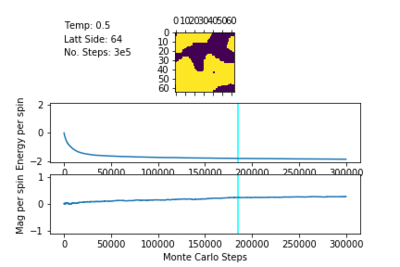
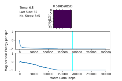
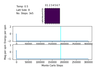
Below the Curie Temperature, $T_{C}$ , the energetic driving force dominates the entropic driving force, resulting in a highly ordered system and an overall magnetisation. The spins of the system align in order to maximise favourable coupling interactions rather than adopting a less ordered configuration of higher multiplicity. Therefore, when $T < T_{C}$ , the most probable configurations have an overall magnetisation resulting in $⟨ M ⟩ \neq 0$ .

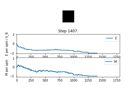
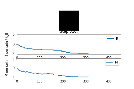
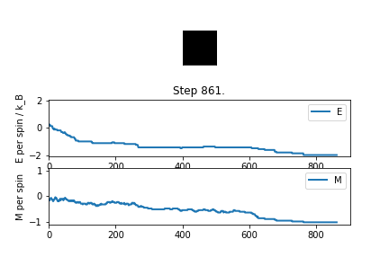
The plots of magnetisation per spin and energy per spin obtained from ILanim.py support this prediction. Below, the plots show that upon equilibration, the system adopts the minimum energy per spin: $E_{m i n_{s p i n}} = \frac{- N D J}{N} = - D J = - 2$ and exhibits the maximum magnitude of magnetisation per spin: $| M_{s p i n} | = 1$

An unknown system error prevented the statistics() function from printing the average values.

Accelerating the Code

Initial Method Speeds

Taking 10 repeat measurements for the time taken to perform 2000 Monte Carlo steps resulted in

An average time of $11.7 s$
A standard error of $0.020 s$

Updating Measurement

NOTE: ILtimetrial.py has been modified to:

Perform a requested number of '2000 Monte Carlo Step' measurements
Record these measurements in a CSV file
Return the mean measuremd time and the Standard Error i.e. $\frac{σ}{n}$

Updating Energy and Magnetisation Methods

Updated Method Speeds

Taking 30 measurements of the time taken to perform 2000 Monte Carlo Steps resulted in:

An average time of $0.87 s$
A standard error of $2.5 \times 1 0^{- 3} s$

This represents a 93% decrease in the average computation time from the initial methods.

The Effect of Temperature

Correcting the Averaging Code

Finding a Delay Value

To quickly find a value for $N_{d}$ , the minimum number of cycles typically needed for the equilibration of a system of within the lattice and temperature ranges of interest, it was assumed that:

Larger lattices would require more Monte Carlo steps to reach equilibrium from their initial, random configurations

Lattices at lower temperatures would require more Monte Carlo steps to reach equilibrium from their initial, random configurations.

Therefore, an initial value for $N_{d}$ was found for a $128 \times 128$ lattice at a temperature of $0.5$ reduced temperature units.

$N_{d} = 185000$

By this number of steps, all smaller lattices at all higher temperatures were found to have equilibrated also. Thus, this value of $N_{d}$ was accepted as an appropriate delay.

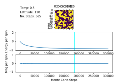
For the 128x128 lattices at T=0.5, equilibration was ensured from 185000 steps onwards.

Smaller lattices at the same temperature did indeed equilibrate more slowly, but all equilibrated within $N_{d}$ MC steps.

The figure below shows the modifications made to IsingLattice.py to incorporate the $N_{d}$ step delay.

Running over a Range of Temperatures

To examine the effect of temperature on the average energy $⟨ E ⟩$ and average magnetisation $⟨ M ⟩$ of Ising lattices at equilibrium, the following parameters were used:

Temperature Range: $0.5 - 5$ reduced units
Temperature Interval: $0.01$ reduced units ( $450$ temperature values)
Number of MMC Steps per Temperature value: $2 \times 1 0^{5}$ with the aforementioned value of $N_{d} = 1.85 \times 1 0^{5}$ Monte Carlo steps
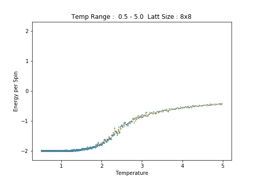
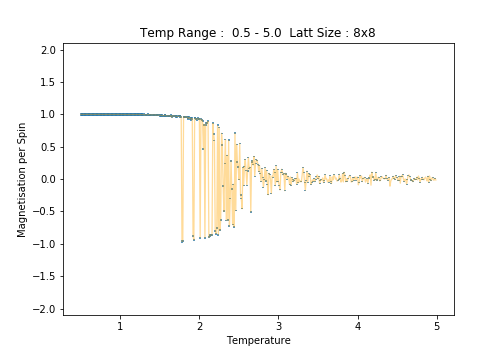
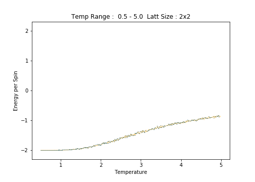
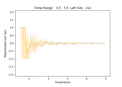
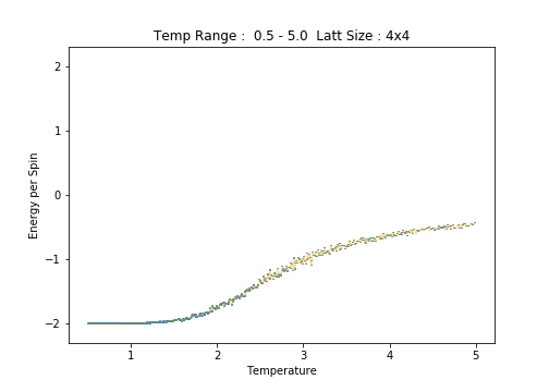
Lattice Sizes: $2 \times 2$ , $4 \times 4$ , $8 \times 8$ , $16 \times 16$ , $32 \times 32$ , $64 \times 64$

Plots of $⟨ E ⟩$ and $⟨ M ⟩$ per spin as versus temperature are presented below for each lattice size. Errorbars have been implemented to demonstrate how well-behaved lattice systems of each size are at each temperature, that is, how temperature and lattice size affect the size of the variations in the expected values. For the error calculations, the standard errors, $σ_{\bar{X}}$ , in $⟨ E ⟩$ and $⟨ M ⟩$ per spin have been used:

8x8

A Python script has been written to generate a plot of $⟨ E ⟩$ or $⟨ M ⟩$ against temperature based upon user input. A screenshot of this code has been inserted below.

The Effect of System Size

Scaling the System Size

More Lattice Sizes

2x2

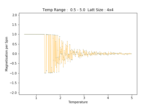
4x4

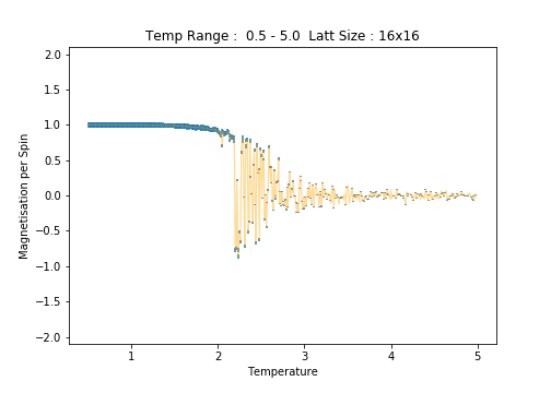
16x16

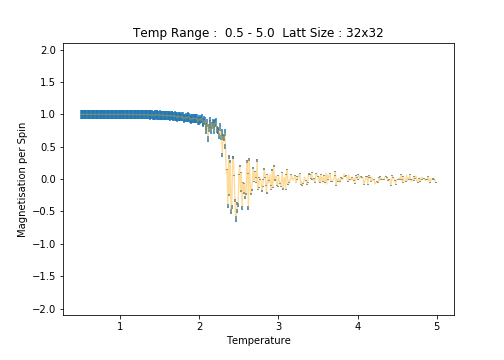
32x32

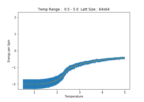
64x64

Scrutiny of the plots of average energy per spin for each lattice size reveals an increase in the errorbar width with increasing lattice size. This is most notable in the low temperature region of the plots. Between the $8 \times 8$ and $16 \times 16$ lattices, the long range fluctuations become suddenly prominent. The $16 \times 16$ lattice is the first (in the range of sizes tested)to clearly capture these fluctuations.

Determining the Heat Capacity

Calculating the Heat Capacity

Heat Capacity Derivation

Working in the canonical ensemble (constant volume), the heat capacity $C_{V}$ is given by:

C_{V} = {\frac{\partial ⟨ E ⟩}{\partial T}}_{V}

where $⟨ E ⟩$ is the average total energy or expected value of the internal energy of the system.

⟨ E ⟩ = - \frac{\partial l n Q}{\partial β} = - \frac{1}{Q} \frac{\partial Q}{\partial β}

where $Q$ is the partition function for the system of N interacting spins.

By evaluating the second form of the partial derivative with respect to $β$ :

$⟨ E ⟩ = - \frac{1}{Q} \frac{\partial Q}{\partial β} = \frac{Σ ϵ_{i} e^{- β ϵ_{i}}}{Σ e^{- β ϵ_{i}}}$

Applying the product rule enables the differentiation of this expression for $⟨ E ⟩$ with respect to temperature, giving:

$\frac{\partial ⟨ E ⟩}{\partial T} = \frac{Σ ϵ_{i} \frac{ϵ_{i}}{k_{B} T^{2}} e^{- β ϵ_{i}}}{Σ e^{- β ϵ_{i}}} - \frac{Σ ϵ_{i} e^{- β ϵ_{i}} \cdot \frac{ϵ_{i}}{k_{B} T^{2}} e^{- β ϵ_{i}}}{(Σ e^{- β ϵ_{i}})^{2}}$

$\frac{\partial ⟨ E ⟩}{\partial T} = \frac{1}{k_{B} T^{2}} [\frac{Σ ϵ_{i}^{2} e^{- β ϵ_{i}}}{Σ e^{- β ϵ_{i}}} - {(\frac{Σ ϵ_{i} e^{- β ϵ_{i}}}{Σ e^{- β ϵ_{i}}})}^{2}]$

$\frac{\partial ⟨ E ⟩}{\partial T} = \frac{1}{k_{B} T^{2}} [⟨ E^{2} ⟩ - {⟨ E ⟩}^{2}]$

Thus,

$\frac{\partial ⟨ E ⟩}{\partial T} = \frac{V a r [E]}{k_{B} T^{2}}$

Heat Capacity versus Temperature

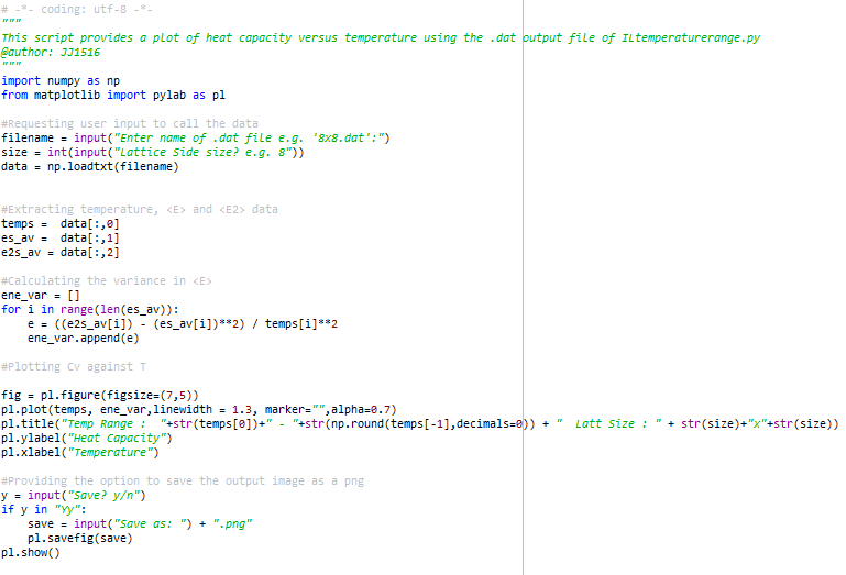
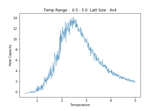
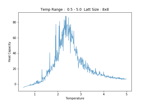
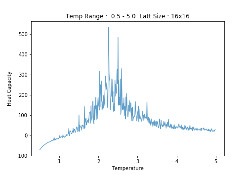
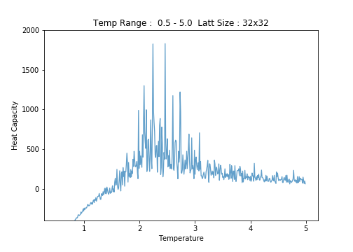
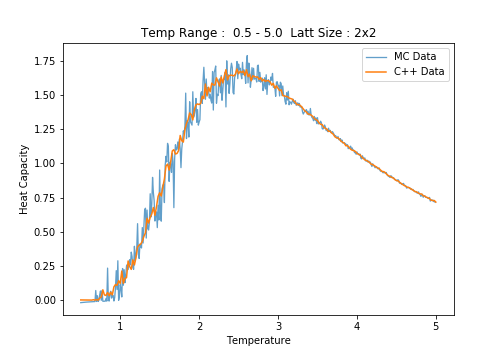
Below, a screenshot of the Python script written to produce plots of $C_{V}$ against $T$ , together with the output images of this script.

2x2

4x4

8x8

16x16

32x32

Locating the Curie Temperature

C++ Data Comparison

Below a comparison of the $C_{V}$ against $T$ plot generated for the $2 / t i m e s 2$ to the corresponding C++ data is offered.

The data generated by the ILtemperaturerange.py script is a faithful match to the C++ data. However, this is an exceptional case; the plots for all other lattice sizes were found to be very dissimilar, necessitating polynomial fitting.

Polyfitting of C++ Data

Fitting a Polynomial to the Entire Range

The following Python script was written to perform a polynomial fit to the entire range of the graph of $C_{V}$ against $T$ .

Below, the result of the polyfit to the $2 / t i m e s 2$ lattice data is offered (for comparison to the previous, non-fitted example).

Polynomials with 5 terms and above were found to match the data in the vicinity of the critical region considerably well. Below 7 terms, the tails of the plot were matched poorly. In the above example, a polynomial of 15 terms was fit to the data.

Fitting a Polynomial to the Critical Region

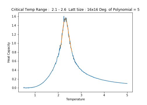
The following Python script was written to perform a polynomial fit to the region of interest (the critical region) of the plots of $C_{V}$ against $T$ to facilitate the discovery of $T_{C}$ .

An example of the result returned by the script is offered below for the C++ data for the $16 \times 16$ lattice.

Finding the Peak C Values for Each Lattice Size

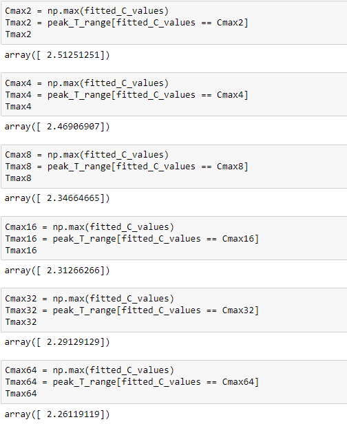
Below, a screenshot of the code used to obtain the temperatures at which the maximum values of C occured is presented for each lattice size. The temperatures themselves are also featured on the image.

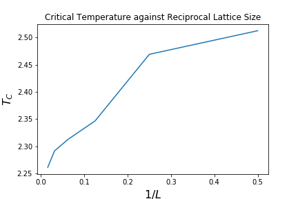
The range of lattice sizes and their associated $T_{C}$ values were exported to a text file, enabling a plot to be created.

Subsequently, the scipy.optimize.curve_fit function was used to fit $T_{C, L} = \frac{A}{L} + T_{C, \infty}$ function to the data obtained. This enabled the estimation the constant $A$ and the value of $T_{C}$ at $\frac{A}{L} = 0$ , otherwise $T_{C, \infty}$ .

A value of $T_{C, \infty} = 2.2799$ was obtained. A comparison to the literature[1] value of $2.269$ reveals a percentage error value of only $0.47 %$ . Surprisingly, the investigation of lattices in the given size range was enough to capture the theoretical behaviour of an infinite lattice. As explained by Frenkel and Smit, the implementation of periodic boundary conditions enables the simulation of an infinite bulk (or infinite adjacent lattices) surrounding the single lattice under scrutiny. The agreement of the experimental and theoretical values for $T_{C, \infty}$ prove the effectiveness of this idea.

A likely source of error arises from the polynomial fitting of the data. The peaks in $C_{V}$ against $T$ were far more sharp than the broad peaks of the polynomial functions used to fit them. In several cases, the polynomial peak was a slight, yet discernible overestimate of the true peak. This has resulted in an overestimation of the final $T_{C, \infty}$ value. Fitting a function with a sharper peak (e.g. a Kronecker delta function) to the critical region could overcome this overestimation and provide a more faithful final value.

References

Frenkel, Daan, et al. Understanding Molecular Simulation : From Algorithms to Applications, Elsevier Science & Technology, 2001

Krieger, M. Constitutions of matter : Mathematically modeling the most everyday of physical phenomena. Chicago ; London: University of Chicago Press, 1996

https://en.wikipedia.org/wiki/Square-lattice_Ising_model Accessed 13-11-18