Rep:JGH116-CMP-Prog

Introduction to the Ising Model

The Ising Model was introduced by Wilhelm Lenz in 1920 as a problem to his student, Ernst Ising, to model ferromagnetism in statistical mechanics. Ferromagnetism is the strongest type of magnetism that exists and is responsible for the phenomena of permanent magnets. A material can be described as ferromagnetic is if exhibits 'spontaneous magnetisation', i.e. it has a net magnetic moment in the absence of an external field. This occurs if the magnetic domains (regions in which the spins of large numbers of unpaired electrons are parallel) in a material align.

The Ising Model is incredibly versatile, and can be used to describe Ionic Liquids, Lattice Gases, and can even be applied in neuroscience. Here, we use the Ising Model as a pedagogical tool to understand the Metropolis Monte Carlo algorithm.

Figure 1: Illustration of an Ising lattice in one (N=5), two (N=5x5), and three (N=5x5x5) dimensions. Red cells indicate the "up" spin", and blue cells indicate the "down" spin.

The Ising Model is based on an 'Ising' Lattice. Consider a set of lattice sites, each with their own neighbours which form a d-dimensional lattice. At each site, there is a discrete variable, s, which represents the 'spin' of the sites, where s ∈ {+1, -1}.

For any two adjacent spins s_i, s_j, there is an interaction energy J_ij ∀ i,j. The total internal energy for a given configuration of spins, $\alpha$, is given by:

$E_{\alpha }=-\sum _{⟨ij⟩}{J}_{ij}{s}_i{s}_j$                    [1]

where ⟨i j⟩ denotes a distinct pair of adjacent spins, with spins s_i, s_j. Assuming that all pairs of spins s_i, s_j, have the same interaction energy, then it is possible to set J_ij = J ∀ ⟨i j⟩ ∈ ⍺. The total internal energy can therefore be rewritten as:

$$\begin{gathered} E_{\alpha }=-\frac{1}{2}J\sum _i^N\sum _{j \\ \in \\ \mathrm{a}\mathrm{d}\mathrm{j}\left(i\right)}{s}_i{s}_j \end{gathered}$$                    [2]

where j ∈ adj(i) denotes every spin j adjacent to spin i. The factor of ½ is included to account for the double counting of interactions in the sum. It is important to note that spins on the edge of the lattice 'wrap around' to interact with the spin on the opposite side of the lattice, making the lattice periodic in space.

TASK: Show that the lowest possible energy for the Ising model is $$\begin{gathered} E \\ = \\ -DNJ \end{gathered}$$, where $D$ is the number of dimensions and $N$ is the total number of spins. What is the multiplicity of this state? Calculate its entropy.

For a 1D lattice, the number of neighbours, N_j, for a given spin i is 2. For a 2D lattice, the number of neighbours is 4, and for a 3D lattice, the number of neighbours is 6. Therefore, the number of neighbours for any given spin i is 2D, where D is the number of dimensions.

The lowest energy configuration is when all spins are parallel, i.e. s_i = s_j = ±1 ∀ i, j. Therefore, the product of any two spins in this configuration is always equal to 1 (s_i * s_j = 1):

$$\begin{gathered} E_{\alpha }=-\frac{1}{2}J\sum _i^N\sum _{j \\ \in \\ \mathrm{a}\mathrm{d}\mathrm{j}\left(i\right)}{s}_i{s}_j \end{gathered}$$ $=-\frac{1}{2}J\sum _i^{N}2D*1$ $=-\frac{1}{2}J*N*2D$ $=-DNJ$                    [3]

The entropy for a given state is given by Boltzmann's equation:

$S_{\alpha }=k_b\ln ({\mathrm{\Omega }}_{\alpha })$                    [4]

where k_b is Boltzmann's constant (1.381 x 10²³ J K^-1), and Ω_⍺ is the multiplicity of the state.

For a state containing N spins, the multiplicity of the state, Ω, is given by:

$\mathrm{\Omega }=\frac{N!}{n_{\uparrow }!n_{\downarrow }!}$                    [5]

where n_↑,↓ is the number of spin up and spin down sites respectively, such that n_↑ + n_↓ = N. For degenerate states, the multiplicity must be adapted to account for this. This can be done by multiplying the multiplicity by the degeneracy:

${\mathrm{\Omega }}_{\alpha }=g_{\alpha }\frac{N!}{n_{\uparrow }!n_{\downarrow }!}$                    [6]

where Ω_⍺, g_⍺ are the multiplicity and the degeneracy of a given configuration ⍺.

For a state where all the spins are parallel, it is doubly degenerate (g_⍺ = 2), as all spins can either be up (N = n_↑) or all spins are down (N = n_↓). Therefore the multiplicity is:

${\mathrm{\Omega }}_{\alpha }=g_{\alpha }\frac{N!}{n_{\uparrow }!n_{\downarrow }!}$ $=2\frac{N!}{n_{\uparrow }!}$ $=2*1=2$

Therefore, the entropy of the lowest energy state is:

$S_{\alpha }=k_b\ln (2)$

Phase Transitions

TASK: Imagine that the system is in the lowest energy configuration. To move to a different state, one of the spins must spontaneously change direction ("flip"). What is the change in energy if this happens ($$\begin{gathered} D=3, \\ N=1000 \end{gathered}$$)? How much entropy does the system gain by doing so?

Figure 2: Illustration showing the energy change when one spin is flipped in the lowest energy configuration of an Ising Lattice.

As shown in figure 2, the number of interactions one spin has is in 3D is six - i.e. it interacts with each of its neighbours. When all the spins are parallel as in the lowest energy configuration, the relative total interaction energy is -6J. When that spin is removed, that interaction energy is lost, taking the total energy up to 0J. If that spin is replaced, pointing down instead of up, then there are only unfavourable interactions, bringing the total energy up to +6J. Therefore, the overall energy change by flipping one spin in the lowest energy configuration in 3D is 12J.

For a 3D system with 1000 spins, the lowest energy configuration has a total energy of:

$E=-DNJ=-3\times 1000\times J=-3000J$

By flipping one spin in this system, there will be an energy change of +12J. Therefore the total energy after flipping will be:

$-3000J+12J=-2988J$

As there are 1000 spins in the system, any one of these can be flipped. Therefore, the multiplicity of this new configuration is:

$\mathrm{\Omega }=\frac{N!}{n_{\uparrow }!n_{\downarrow }!}=\frac{1000!}{999!1!}=1000$

However, there are 2 degenerate states (999 up, 1 down and 1 up, 999 down), and so the total multiplicity is:

${\mathrm{\Omega }}_{\alpha }=g_{\alpha }\frac{N!}{n_{\uparrow }!n_{\downarrow }!}=2\times 1000=2000$

Therefore, the entropy of this state is:

$S_{\alpha }=k_b\ln ({\mathrm{\Omega }}_{\alpha })=k_b\ln (2000)$

The change in entropy between this state and the lowest energy configuration is therefore:

$\mathrm{\Delta }S=S_f-S_i=k_b\ln (2000)-k_b\ln (2)=k_b\ln \left(\frac{2000}{2}\right)=k_b\ln (1000)=9.5371821\times 10^{-23}J{K}^{-1}$

TASK: Calculate the magnetisation of the 1D and 2D lattices in figure 1. What magnetisation would you expect to observe for an Ising lattice with $$\begin{gathered} D=3, \\ N=1000 \end{gathered}$$ at absolute zero?

Magnetisation, M, is given by the following equation:

$M=\sum _i^N{s}_i$                    [7]

where s_i is the spin of a given spin i ∈ N. From the lattices in figure 1, the respective magnetisations are:

$1D:M=3\times (+1)+2\times (-1)=1$

$2D:M=13\times (+1)+12\times (-1)=1$

The Free Energy of a system is always looking to be minimised, i.e. as low as possible. The Helmholtz Free energy, F, is given by the following equation:

$F=U-TS$                    [8]

where U is the internal energy, T is the temperature, and S is the entropy. When $T=0$, the system is in its lowest energy state. The entropy of this state is $S=k_b\ln (2)$. However, the entropic contribution to the free energy is 0 $(T\times S=0)$. Therefore, the only contribution to the free energy is the internal energy, which we know is minimised when all spins are parallel. They can either all be pointing up or all be pointing down, and so for a system with $D=3,N=1000$, the magnetisation is:

$M=\sum _i^N{s}_i=\pm \sum _i^{1000}1=\pm 1000$

Calculating the Energy and Magnetisation

TASK: Complete the functions energy() and magnetisation(), which should return the energy of the lattice and the total magnetisation, respectively. In the energy() function you may assume that $J=1.0$ at all times (in fact, we are working in reduced units in which $J=k_b$, but there will be more information about this in later sections). Do not worry about the efficiency of the code at the moment — we will address the speed in a later part of the experiment.

To calculate the energy, the sum of the spin of every site multiplied by the spin of each of its neighbours is taken, as per [2]. As the lattice is formed using a numpy array, this calculation can be performed using a nested loop to scan through each spin in the lattice. Using indexing, the neighbours of a given spin can be selected, and [2] can be applied. For a spin at the edge of the lattice, indexing using [i+1] or [j+1] would not work, as the index exceeds the size of the array. Therefore, the remainder of [i+1] and [j+1] with respect to the lattice size was taken in order to return the index back to zero for the edge. This was not a problem for [i-1] and [j-1], as the index of [-1] returns the desired element of the array. The following function shows how this was implemented.

def energy(self):
    "Returns the total energy of the current lattice configuration."
    energy=0
    for i in range(0,len(self.lattice)): #for each row
        for j in range(0,len(self.lattice[i])): #for each element
            s0=self.lattice[i][j]
            s1=self.lattice[i][(j+1)%self.n_cols] #taking the remainder
            s2=self.lattice[i][j-1]
            s3=self.lattice[(i+1)%self.n_rows][j] #taking the remainder
            s4=self.lattice[i-1][j]
            energy=energy+s0*s1+s0*s2+s0*s3+s0*s4 
    return -0.5*energy #divide by 2 to account for double counting of interactions

A similar approach was used to calculate the magnetisation. Magnetisation is found from [7], so by scanning through each spin in the lattice and keeping a running sum, this can be calculated. The following function shows how this was implemented.

def magnetisation(self):
    "Return the total magnetisation of the current lattice configuration."
    magnetisation=0
    for i in self.lattice:
       for j in i:
            magnetisation=magnetisation+j
    return magnetisation

Figure 3: The result of running the ILcheck.py script - as shown, the actual values of the energy and magnetisation match the expected values.

TASK: Run the ILcheck.py script from the IPython Qt console using the command

%run ILcheck.py

The displayed window has a series of control buttons in the bottom left, one of which will allow you to export the figure as a PNG image. Save an image of the ILcheck.py output, and include it in your report.

When running the ILcheck.py script, the three lattices in figure 3 were produced. These show the lowest energy, random, and highest energy configurations of a 4x4 Ising Lattice, and their expected energies. The energies and magnetisations calculated using the functions written above match the expected values, showing that they work!

Introduction to Monte Carlo simulation

Average Energy and Magnetisation

In statistical mechanics, average value of a property of a system at a given temperature is computed using the following equation:

$⟨X{⟩}_T=\sum _{\alpha }{X}_{\alpha }\rho (\alpha )$                    [9]

where $\rho (\alpha )$ is the probability of the system being in the state $\alpha$. The states in the Ising Model are distributed via a Boltzmann distribution, and therefore, the average values of energy and magnetisation are:

$⟨E{⟩}_T=\frac{1}{Z}\sum _{\alpha }{E}_{\alpha }\exp \{-\frac{E_{\alpha }}{k_{b}T}\}$                    [10]

$⟨M{⟩}_T=\frac{1}{Z}\sum _{\alpha }{M}_{\alpha }\exp \{-\frac{E_{\alpha }}{k_{b}T}\}$                    [11]

where Z is the partition function and $E_{\alpha }$ is the energy of a given configuration, $\alpha$. Although these equations are the definition of the average energy and magnetisation, they are not practical. The partition functions for the 1D and 2D Ising lattices are given below:

$1D:Z(T,N)=[2\cosh \left(\frac{J}{k_{b}T}\right){]}^N$                    [12]

$2D:\underset{N\to \mathrm{\infty }}{\lim }\ln Z(T,N)=\ln (2\cosh \left(2\beta J\right))+\frac{1}{2\pi }\underset{0}{\overset{\pi }{\int }}\ln \frac{1}{2}(1+\sqrt{1-{\kappa }^2{\sin }^2\varphi })d\varphi$                    [13]

where $\kappa =\frac{2\sinh \left(2\beta J\right)}{{\cosh }^2\left(2\beta J\right)}$

For dimensions greater than 2, no analytical solutions are known! Using these to compute the average energies and magnetisations of Ising Lattices both lengthens and complicates the process, and so the problem is tackled using numerical methods, namely the Monte Carlo simulation.

TASK: How many configurations are available to a system with 100 spins? To evaluate these expressions, we have to calculate the energy and magnetisation for each of these configurations, then perform the sum. Let's be very, very, generous, and say that we can analyse $1\times 10^9$ configurations per second with our computer. How long will it take to evaluate a single value of ${⟨M⟩}_T$?

For each spin, there are 2 possible configuration, either spin up or spin down. If there were 100 spins in a system, the total number of configurations available for that system would be 2¹⁰⁰ = 1267650600228229401496703205376 configurations. Assuming a computer can analyse 10⁹ of these configurations per second, a single value of $⟨M{⟩}_T$ would take:

$=\frac{2^{100}}{10^9}=1.2676506002282295\times 10^{21}s$

To put this into perspective, this is equivalent to approx. 40196937 million years! This is obviously not a practical solution. Instead, we can consider [10] & [11]. The majority of the states in the system will have a very small Boltzmann weighting factor $\exp \{E_{\alpha }/k_{b}T\}$ and so will not contribute much to the overall average energy. Instead, if only the states with sizeable Boltzmann weighting factors are considered, then an enormous amount of time can be saved. This is importance sampling - instead of sampling through all the possible states, only the states which the system are likely to occupy are sampled.

Modifying IsingLattice.py

TASK: Implement a single cycle of the Monte Carlo algorithm in the montecarlocycle(T) function. This function should return the energy of your lattice and the magnetisation at the end of the cycle. You may assume that the energy returned by your energy() function is in units of $k_B$! Complete the statistics() function. This should return the following quantities whenever it is called: $⟨E⟩,⟨E^2⟩,⟨M⟩,⟨M^2⟩$, and the number of Monte Carlo steps that have elapsed.

The Metropolis Monte Carlo algorithm is as follows:

1. Start from a given configuration of spins, ${\alpha }_0$, with energy $E_0$.
2. Choose a single spin at random, and "flip" it, to generate a new configuration ${\alpha }_1$
3. Calculate the energy of this new configuration, $E_1$
4. Calculate the energy difference between the states, $\mathrm{\Delta }E=E_1-E_0$
   1. If the $\mathrm{\Delta }E<0$ (the spin flipping decreased the energy), then we accept the new configuration.
      • We set ${\alpha }_0={\alpha }_1$, and $E_0=E_1$, and then go to step 5
   2. If $\mathrm{\Delta }E>0$, the spin flipping increased the energy. By considering the probability of observing the starting and final states, ${\alpha }_0$ and ${\alpha }_1$, it can be shown that the probability for the transition between the two to occur is $\exp \{-\frac{\mathrm{\Delta }E}{k_{B}T}\}$. To ensure that we only accept this kind of spin flip with the correct probability, we use the following procedure:
      1. Choose a random number, $R$, in the interval $[0,1)$
      2. If $R\le \exp \{-\frac{\mathrm{\Delta }E}{k_{B}T}\}$, we accept the new configuration.
         • We set ${\alpha }_0={\alpha }_1$, and $E_0=E_1$, and then go to step 5
      3. If $R>\exp \{-\frac{\mathrm{\Delta }E}{k_{B}T}\}$, we reject the new configuration.
         • ${\alpha }_0$ and $E_0$ are left unchanged. Go to step 5
5. Update the running averages of the energy and magnetisation.
6. Monte Carlo "cycle" complete, return to step 2.

This algorithm was implemented in the function below. There are three possible routes in this algorithm:

1. $\mathrm{\Delta }E<0$ and the new configuration is accepted
2. $\mathrm{\Delta }E>0$ and the new configuration is accepted
3. $\mathrm{\Delta }E>0$ and the new configuration is rejected

Since routes 1 and 2 end in the same result, and only route 3 ends in a rejection of the new configuration, only one 'if' statement is required. This can be seen in the code below. Once the new state is either accepted or rejected, the energy, energy squared, magnetisation and magnetisation squared of the new state is added to the variables defined in the IsingLattice constructor also shown below:

def __init__(self, n_rows, n_cols):
    self.n_rows = n_rows
    self.n_cols = n_cols
    self.lattice = np.random.choice([-1,1], size=(n_rows, n_cols))
    self.E=0
    self.E2=0
    self.M=0
    self.M2=0
    self.n_cycles=0   

def montecarlostep(self, T):
    "Performs one step of the Monte Carlo simulation"
    self.n_cycles+=1   #Increases the counter recording the number of Monte Carlo steps performed 
    e_i = self.energy()
    #the following two lines selects the coordinates of a random spin in the lattice
    random_i = np.random.choice(range(0, self.n_rows))
    random_j = np.random.choice(range(0, self.n_cols))
    #the following line flips the randomly selected spin 
    self.lattice[random_i][random_j]=-1*self.lattice[random_i][random_j]
    e_f=self.energy()
    random_number = np.random.random()
    #the following line is the condition for which the new configuration is rejected
    if e_f>e_i and random_number > np.exp(-(e_f-e_i)/T):
        self.lattice[random_i][random_j]=-1*self.lattice[random_i][random_j]
        mag=self.magnetisation()
        self.E=self.E+e_i
        self.E2=self.E2+e_i**2
        self.M=self.M+float(mag)
        self.M2=self.M2+float(mag)**2
        return float(e_i), float(mag)
    else:
        mag=self.magnetisation()
        self.E=self.E+e_f
        self.E2=self.E2+e_f**2
        self.M=self.M+float(mag)
        self.M2=self.M2+float(mag)**2
        return float(e_f), float(mag)

After a set of Monte Carlo steps, the E, E², M and M² values from each step will have been summed up. To calculate the average quantities, the values are divided by the number of Monte Carlo steps taken. The statistics() function below shows this calculation.

 def statistics(self):
     "Returns the average E, E^2, M, M^2 and the number of Monte Carlo steps performed" 
     E=self.E/self.n_cycles
     E2=self.E2/self.n_cycles
     M=self.M/self.n_cycles
     M2=self.M2/self.n_cycles
     return E,E2,M,M2, self.n_cycles

This algorithm enables the minimisation of free energy, despite using just the calculated internal energy. However, as shown in [8], there is also an entropic contribution to the free energy. So how is this method accounting for the entropy contribution?

By involving the Boltzmann factor as the probability factor, this means the accepted states are distributed via the Boltzmann distribution. By randomly flipping a spin, there is a probability that a higher energy state can be accepted. By accepting this higher energy state, it enables fluctuations about the equilibrium state. The underlying distribution of these states around the equilibrium state would be a Gaussian. Being able to access these states accounts for the entropy. An easy way to see this is by considering the system at a very high temperature. As T increases, more and more configurations become accessible, and the Boltzmann distribution flattens. Consequently, the multiplicity $\mathrm{\Omega }\to 2^N$, and hence $S\to k_b\ln (2^N)$, where N is the number of spins, as $T\to \mathrm{\infty }$. As a Monte Carlo step is applied on the system, it is significantly more likely for a higher energy configuration to be accepted at a high temperature, because the Boltzmann factor $\exp \left\{\frac{E_{\alpha }}{k_{b}T}\right\}\to 1$ as $T\to \mathrm{\infty }$, which corresponds with the multiplicity, $\mathrm{\Omega }$, of the system, and hence, the entropy. Thus, this method accounts for the entropy.

Figure 4: The result of running the ILanim.py script for an 8x8 lattice at a temperature of 0.5, producing: a) a lowest energy configuration of the lattice b) a metastable state

Figure 5: The result of running the ILanim.py script for an 8x8 lattice at a temperature of 15, producing fluctuations about E,M=0

TASK: If $T<T_C$, do you expect a spontaneous magnetisation (i.e. do you expect $⟨M⟩\ne 0$)? When the state of the simulation appears to stop changing (when you have reached an equilibrium state), use the controls to export the output to PNG and attach this to your report. You should also include the output from your statistics() function.

The Curie Temperature is defined as the temperature above which a material loses their permanent magnetic properties. Therefore, below the Curie Temperature, i.e. $T<T_C$ spontaneous magnetisation is expected.

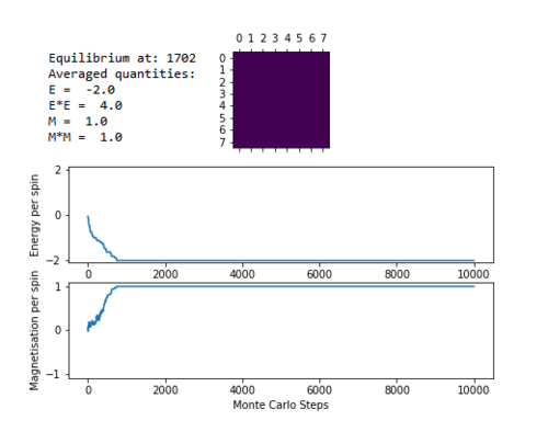
The animation script ILanim.py was run for an 8x8 lattice at a temperature of 0.5. Once the simulation stopped changing energy, i.e. once it had reached an equilibrium state, a screenshot of the graph and the averaged values was taken.

Each simulation begins with a random lattice, and performs Monte Carlo steps on it. The first simulation performed is shown in figure 4. This shows the system lowering its energy with each Monte Carlo step, reaching the lowest energy configuration at around step 700. Once the system has reached this configuration, it does not fluctuate from it, and it remains there, i.e. it has reached equilibrium. The energy per spin in the lowest energy configuration is -2, and the magnetisation per spin is 1. The averaged quantities, however, do not discard the initial minimisation steps, and so takes them into account when calculating the average. This is why the averaged quantities for E and M are significantly different to -2 and 1 respectively.

The simulation was run again under the same conditions, with an 8x8 lattice at a temperature of 0.5. This time, however, the system reached an equilibrium in a metastable state (see figure 5). This is when the system is kinetically stable, but not in its lowest energy state. Instead, it is stuck in a local minimum instead of the global minimum. The mechanical 'thermal' fluctuation applied by the Monte Carlo algorithm is not enough for the system to kick itself out of this state. However, if a stronger 'kick' is applied, the system will free itself from this metastable state. Therefore, despite being stable, the system is not in equilibrium. Examples of metastable states in reality are Diamond, or supercooled water. In this system, there is still an overall magnetisation, as there are more spin up spins than spin down spins.

The simulation was run yet again with the same lattice size, but at a much higher temperature of 15 to ensure $T>T_C$. It is immediately obvious that at a high temperature there are significantly more fluctuations (see figure 6). However, these fluctuations are all around an 'equilibrium' of $E,M=0$. As described above, the states around the equilibrium state are distributed via a Gaussian distribution. As a consequence of this distribution, the magnitude of these fluctuations from the equilibrium is estimated to be $\approx \frac{1}{\sqrt{N}}$. As $N=64$ here, the magnitude of the fluctuation would be approximately $1/8=0.125$. As seen in figure 6, this seems to be the case, validating the claim that there is an underlying Gaussian distribution.

The fluctuations in magnetisation here are all happening around $M=0$. It is therefore reasonable to assume that a temperature of 15 is greater than the Curie temperature. It is possible to conclude that when $T>T_C,⟨M⟩\to 0$.

By performing these three simulations, we show that when $T<T_C$, there is spontaneous magnetisation, and when $T>T_C$, the system loses most, if not all of its magnetic properties.

Accelerating the code

TASK: Use the script ILtimetrial.py to record how long your current version of IsingLattice.py takes to perform 2000 Monte Carlo steps. This will vary, depending on what else the computer happens to be doing, so perform repeats and report the error in your average!

The python script ILtimetrial.py was run 16 times, giving the following runtimes for 2000 Monte Carlo steps (to 12 d.p.):

	1	2	3	4	5	6	7	8
Runtime (s)	5.75730054321	5.81583604945	5.72269787654	6.06356069136	5.69132167910	5.99814558025	5.75052444444	5.59712908642
	9	10	11	12	13	14	15	16
Runtime (s)	5.77942953086	5.84957432099	6.40311703704	5.43301412346	5.69427753156	6.01423604938	5.88791506173	5.89307417284

From these values, the average runtime for 2000 Monte Carlo steps is:

$t=5.83444711111\pm 0.21330451356s$

TASK: Look at the documentation for the NumPy sum function. You should be able to modify your magnetisation() function so that it uses this to evaluate M. The energy is a little trickier. Familiarise yourself with the NumPy roll and multiply functions, and use these to replace your energy double loop (you will need to call roll and multiply twice!).

The numpy.sum() function sums all the elements in an array. As the calculation for magnetisation, M, involves summing up all the spins, this sum function can be applied to the lattice, as shown below:

def magnetisation(self):
    "Return the total magnetisation of the current lattice configuration."
    return 1.0*np.sum(self.lattice)

The numpy.multiply() function multiplies each element in an array with the corresponding element in another array. The numpy.roll() function enables the shifting of rows up and down and columns left and right in the array. By combining these two functions together, as well as the sum function, it is possible to calculate the energy of the lattice. Multiplying the lattice by a lattice rolled once to the right takes into account all interactions between each spin and its neighbour to the left. Multiplying the lattice by a lattice rolled once downwards takes into account all interactions between each spin and its neighbour above. This counts every interaction in the lattice without double counting. By applying the sum function to these lattices, and adding the resulting sums together, you calculate the energy. The code for this is shown below:

def energy(self):
    "Return the total energy of the current lattice configuration."
    il=self.lattice
    return -1.0*np.sum(np.multiply(il, np.roll(il, 1, 0)))-1.0*np.sum(np.multiply(il, np.roll(il, 1, 1)))

TASK: Use the script ILtimetrial.py to record how long your new version of IsingLattice.py takes to perform 2000 Monte Carlo steps. This will vary, depending on what else the computer happens to be doing, so perform repeats and report the error in your average!

After implementing these new functions for energy and magnetisation, the runtime was shortened significantly, as shown by the following table:

	1	2	3	4	5	6	7	8
Runtime (s)	0.514644938272	0.3674540246914	0.3432410864198	0.397299753086	0.3896584691358	0.342273185185	0.3765925925925	0.325619753086
	9	10	11	12	13	14	15	16
Runtime (s)	0.3554710123456	0.327868049383	0.3836053333332	0.4080521481483	0.3602054320988	0.317112888889	0.358967703704	0.339137975309

From these values, the average runtime for 2000 Monte Carlo steps is:

$t=0.369200271605\pm 0.0455071720835s$

This is almost 16 times faster than the previous code!

Phase Behaviour of the Ising Model

Correcting the Averaging Code

Figure 6 A gif showing how the number of Monte Carlo steps required for equilibrium increases with lattice size.

Figure 7 A gif showing how the energy and magnetisation as functions of number of Monte Carlo steps vary with temperature.

Figure 8 A simulation of a 100x100 lattice at a temperature of 0.01. The 'phase' separation visible here is analogous to Spinodal Decomposition.

TASK: The script ILfinalframe.py runs for a given number of cycles at a given temperature, then plots a depiction of the final lattice state as well as graphs of the energy and magnetisation as a function of cycle number. This is much quicker than animating every frame! Experiment with different temperature and lattice sizes. How many cycles are typically needed for the system to go from its random starting position to the equilibrium state? Modify your statistics() and montecarlostep() functions so that the first N cycles of the simulation are ignored when calculating the averages. You should state in your report what period you chose to ignore, and include graphs from ILfinalframe.py to illustrate your motivation in choosing this figure.

Figure 6 shows the result of running the python script ILfinalframe.py with increasing lattice sizes. It can be seen that the number of Monte Carlo steps required for the system to reach equilibrium increases with lattice size. For an 8x8 system, only around 400 steps are required. For a 15x15 system, this increased to around 5000 steps. When the lattice size was increased to 30x30 and 50x50, this increased rapidly to 750000 and 950000 steps respectively.

Figure 7 shows the result of running the python script ILfinalframe.py with an 8x8 lattice and increasing temperature. As the temperature increases, the energy and magnetisation begin to fluctuate about the lowest energy. Once T=2, the fluctuations begin to increase even further. At T=3 & T=5, the energy fluctuates around E,M=0. This shows that the Curie Temperature, $T_C$, is between 2 and 3 for the 8x8 system.

The code was run again for a 100x100 system at a temperature of 0.01 with 1 million Monte Carlo steps. The result of this simulation is shown in figure 8. Similar to the metastable state described above, there are defined domains of parallel spins, which have a net magnetisation. This shows an example of spinodal decomposition. This is normally applied to the unmixing of a mixture of liquids or solids in one thermodynamic phase to form two coexisting phases. Here, the two different spins (spin up or spin down) can be considered as different phases. At the beginning of the simulation, the distribution of spins is random, much like a mixture of two phases. As Monte Carlo steps are applied (analogous to cooling the system), these spins 'unmix' in order to reduce the free energy, i.e. clusters of the same spin start to form as there is no energy barrier to the nucleation of the 'spin up'-rich and 'spin down'-rich phases. As the lattices are periodic, they can be tiled, which emphasises these clusters of different phases.

From above, it can be seen that the number of steps taken to reach equilibrium varies with lattice size and temperature. If the averaging code were to be adapted to start recording data to average after $x$ number of steps, it would not be possible to state a number $x$ that applies for all situations, i.e. as stated before, $x$ varies depending on temperature and lattice size. In order to get around finding this relationship between $x$, lattice size and temperature, general conditions for equilibrium were considered. In any system, equilibrium occurs when the system is stable in a global minimum. As seen in previous figures, this is when the average energy remains constant. To find the point at which this occurs, the initial algorithm used was as follows:

1. Set a 'checking' variable as False at the beginning of the simulation - once the system has reached equilibrium, this will be changed to True.
2. Once enough steps have been taken at a point $a$, a sample of data of size $w$ is taken, i.e. data from the point $a-w$ to $a$ is taken as the sample.
3. The standard deviation of this sample is taken:
   • If this standard deviation is lower than the predefined 'threshold' value, the system is in equilibrium, and the checking variable is set to True, a new step counter is started, and the relevant statistics variables begin to record data with the subsequent Monte Carlo steps.
   • If this standard deviation is higher than the predefined 'threshold' value, checking variable remains set to False, the next Monte Carlo step is taken and the sample moves along.

This algorithm worked for small lattices and low temperatures. However, at high temperature, even though the system had reached equilibrium, the energy fluctuated significantly more than our standard deviation threshold would allow. Therefore, the algorithm had to be adapted to account for these fluctuations. Rather than taking the standard deviation of a single sample of data, the standard deviation of the means of three samples was taken. The initial sample size in the algorithm was split into three separate samples, and the mean of each of these samples were taken. The standard deviation of these means was measured, and if this was below a predefined 'threshold' value the system would be defined as in equilibrium. The algorithm was changed to reflect this:

1. Set a 'checking' variable as False at the beginning of the simulation - once the system has reached equilibrium, this will be changed to True.
2. Once enough steps have been taken at a point $a$, a three samples of data of size $w$ are taken, i.e. three samples from the point $a-3w$ to $a$ are taken, each with size $w$.
3. The means of these three samples are taken, and then the standard deviation of these means is calculated.
   • If this standard deviation is lower than the predefined 'threshold' value, the system is in equilibrium, and the checking variable is set to True, a new step counter is started, and the relevant statistics variables begin to record data with the subsequent Monte Carlo steps.
   • If this standard deviation is higher than the predefined 'threshold' value, checking variable remains set to False, the next Monte Carlo step is taken and the sample moves along.

This algorithm was implemented in the montecarlostep() function, as shown below:

def montecarlostep(self, T):
    "Performs one Monte Carlo step"
    self.n_cycles+=1
    e_i = self.energy()
    #the following two lines select the coordinates of a random spin
    random_i = np.random.choice(range(0, self.n_rows))
    random_j = np.random.choice(range(0, self.n_cols))
    self.lattice[random_i][random_j]=-1*self.lattice[random_i][random_j]
    e_f=self.energy()
    random_number = np.random.random()
    #the following line defines the sample size
    weight=self.n_rows*self.n_cols*5
    #this 'if' statement performs the equilibrium check, only if the system is not in equilibrium 
    if self.n_cycles>3*weight and self.check==False:
        mean1=np.mean(np.array(self.elist[self.n_cycles-3*weight:self.n_cycles-2*weight]))
        mean2=np.mean(np.array(self.elist[self.n_cycles-2*weight:self.n_cycles-weight]))
        mean3=np.mean(np.array(self.elist[self.n_cycles-weight:self.n_cycles]))
        sample=np.array([mean1,mean2,mean3])  
        if np.std(sample)<0.01*T: #if the standard deviation is smaller than this temp. dependent threshold variable, the system is in equilibrium
            self.check=True   #redefine the checking variable to show the system is in equilibrium
            print('Equilibrium at:', self.n_cycles)
    if e_f>e_i and random_number > np.exp(-(e_f-e_i)/T):
        self.lattice[random_i][random_j]=-1*self.lattice[random_i][random_j]
        self.elist.append(e_i)
        mag=self.magnetisation()
        self.mlist.append(mag)
        #This 'if' statement is added so that the statistics variables will only start recording data when the system is in equilibrium
        if self.check==True: 
            self.n_threshold+=1
            self.E=self.E+e_i
            self.E2=self.E2+e_i**2
            self.M=self.M+float(mag)
            self.M2=self.M2+float(mag)**2
        return float(e_i), float(mag)
    else:
        mag=self.magnetisation()
        self.elist.append(e_f)
        self.mlist.append(mag)
        if self.check==True:
            self.n_threshold+=1
            self.E=self.E+e_f
            self.E2=self.E2+e_f**2
            self.M=self.M+float(mag)
            self.M2=self.M2+float(mag)**2
        return float(e_f), float(mag)

In order to get this code to work, new variables had to be defined in the __init__() function:

def __init__(self, n_rows, n_cols):
    self.n_rows = n_rows
    self.n_cols = n_cols
    self.lattice = np.random.choice([-1,1], size=(n_rows, n_cols))
    self.E=0
    self.E2=0
    self.M=0
    self.M2=0
    self.n_cycles=0
    self.check=False
    self.elist=[]
    self.mlist=[]
    self.n_threshold=0

The statistics function needed to be altered as well in order to account for this - instead of dividing each sum by self.n_cycles, we instead divide by the new counter that begins when the system is defined as being in equilibrium, self.n_threshold.

def statistics(self):   
    E=self.E/self.n_threshold
    E2=self.E2/self.n_threshold
    M=self.M/self.n_threshold
    M2=self.M2/self.n_threshold
    return E,E2,M,M2,self.n_threshold

This algorithm proved to work well when running simulations.

• 
  8x8 Lattice at a temperature of 0.01 for 10000 Monte Carlo Steps.
• 
  8x8 Lattice at a temperature of 5 for 20000 Monte Carlo Steps.

The effect of temperature

TASK: Use ILtemperaturerange.py to plot the average energy and magnetisation for each temperature, with error bars, for an 8 x 8 lattice. Use your intuition and results from the script ILfinalframe.py to estimate how many cycles each simulation should be. The temperature range 0.25 to 5.0 is sufficient. Use as many temperature points as you feel necessary to illustrate the trend, but do not use a temperature spacing larger than 0.5. The NumPy function savetxt() stores your array of output data on disk — you will need it later. Save the file as 8x8.dat so that you know which lattice size it came from.

It was found that the averaging code written was having issues with recording data at high temperature, as the fluctuations became so large that the equilibrium conditions set were never met. Therefore, the statistics() function was modified to include a case for which the system had not been in equilibrium:

def statistics(self):
    "Calculates the correct values for the averages of E,E*E (E2), M, M*M (M2), and returns them"
    if self.check==False: #this checks to see if the system is in equilibrium - if not, then it takes the last 20000 steps
        Earray=np.array(self.elist[self.n_cycles-20000:self.n_cycles])
        E=np.sum(Earray)/20000
        E2=np.sum(np.multiply(Earray,Earray))/20000
        Marray=np.array(self.mlist[self.n_cycles-20000:self.n_cycles])
        M=np.sum(Marray)/20000
        M2=np.sum(np.multiply(Marray,Marray))/20000
        return E,E2,M,M2,20000
    else: 
        E=self.E/self.n_threshold
        E2=self.E2/self.n_threshold
        M=self.M/self.n_threshold
        M2=self.M2/self.n_threshold
        return E,E2,M,M2,self.n_threshold

The python script ILtemperaturerange.py had to be modified to account for the new variables defined in the constructor. After each temperature simulation, all the variables had to be reset:

il.E = 0.0
il.E2 = 0.0
il.M = 0.0
il.M2 = 0.0
il.n_cycles = 0
il.check=False
il.n_threshold=0
il.elist=[]
il.mlist=[]

Figure 9 Graphs showing how the energy and magnetisation vary with temperature for an 8x8 lattice

Running the python script ILtemperaturerange.py performs a series of Monte Carlo steps for increasing temperatures, enabling the plotting of average values with temperature. These plots for an 8x8 system are shown in figure 9. The temperature range was from 0.25 to 5.0, with a temperature spacing of 0.01. This spacing was chosen in order to show the detail, and the level of fluctuation that occurs when criticality is reached.

At low temperatures, the preferred state for the system is the lowest energy state, which has $⟨E⟩=-2$,$⟨M⟩=\pm 1$, i.e. all spins are parallel. As the temperature rises, the state has a net magnetisation, but clusters of opposite spins begin to appear. These clusters have an intrinsic size which increases with temperature, called the correlation length. As the clusters grow, they start to contain smaller, fractal clusters within themselves. As the temperature rises above 2, the system starts to undergo a phase transition, and it reaches the critical point, the Curie Temperature $(T_C)$. At this point, the correlation length diverges, and the entire system turns into a giant cluster, with no net magnetisation. This giant cluster contains smaller sized 'fractal' clusters. While a single perturbation may not affect a large cluster, it can affect the smaller clusters. However, when the smaller clusters are perturbed, they in turn perturb a larger cluster, which in turn perturbs an even larger cluster and so on. Therefore, a small perturbation can greatly affect a system at its critical point. This can be seen in the graphs plotted for energy and magnetisation. The large fluctuations in the average magnetisation show the system approaching its critical point, and once past it, the average magnetisation is zero. A similar observation can be made for the energy, however it is not as pronounced - there are fluctuations in the energy close to the critical point.

Error bars are added to the graphs to give a sense of how much the average energy/magnetisation fluctuates at a given temperature. As expected, the error in energy increases as temperature rises. This is due to randomly flipped spins being more likely to be accepted at a higher temperature, varying the energy even more. The opposite occurs in the magnetisation. As temperature increases, the error bars shrink. This is because the ratio of up and down spins tend to 1:1 at temperature increases. Therefore the magnetisation gets closer to zero, and the error in this reduces consequentially.

The effect of system size

Figure 10 A gif showing how the energy varies with temperature with varying lattice sizes

Figure 11 A gif showing how the magnetisation varies with temperature with varying lattice sizes

TASK: Repeat the final task of the previous section for the following lattice sizes: 2x2, 4x4, 8x8, 16x16, 32x32. Make sure that you name each datafile that your produce after the corresponding lattice size! Write a Python script to make a plot showing the energy per spin versus temperature for each of your lattice sizes. Hint: the NumPy loadtxt function is the reverse of the savetxt function, and can be used to read your previously saved files into the script. Repeat this for the magnetisation. As before, use the plot controls to save your a PNG image of your plot and attach this to the report. How big a lattice do you think is big enough to capture the long range fluctuations?

Figures 10 and 11 show how the variation of energy and magnetisation with temperature varies with lattice size. The temperature range used in ILtemperaturerange.py for all these lattices was from 0.25 to 5.0, with a temperature spacing of 0.01, for the same reasons as before. The first major observation is that the size of the error bars decrease as the lattice gets larger. This is intuitive, as a single spin flip for a larger system with more spins is less likely to affect the average energy than it would for a smaller system.

Secondly, the temperature at which the magnetisation drops increases as the lattice size increases. This can be attributed to long range fluctuations. It is a characteristic of phase transitions that large fluctuations in the system occur over long ranges. This can be seen as the lattice size increases from 2x2 → 16x16. The magnetisation begins to fluctuate drastically at a much lower temperature than the Curie temperature for the 2x2 system, and the temperature at which this fluctuation occurs increases as the lattice size increases. However, the size of the fluctuation also decreases in size as lattice size increases. In the 32x32 lattice simulation, fluctuations only begin to occur once the phase transition begins. Therefore, a lattice size of 16x16 is large enough to capture the long range fluctuations.

Calculating the heat capacity

TASK: By definition,

$C_v=\frac{\partial ⟨E⟩}{\partial T}$

From this, show that

$C_v=\frac{\mathrm{V}\mathrm{a}\mathrm{r}[E]}{k_B{T}^2}$

(Where $\mathrm{V}\mathrm{a}\mathrm{r}[E]$ is the variance in $E$.)

The average energy ⟨E⟩ is defined by the following equation:

$⟨E⟩=\sum _n{E}_n\rho (n)=\frac{\sum _n{E}_n{e}^{-\beta E_n}}{\sum _n{e}^{-\beta E_n}}$

This can be manipulated to give the average energy as a function of the partition function, Z:

$⟨E⟩=\frac{1}{Z}\sum _n{E}_n{e}^{-\beta E_n}$

$=\frac{1}{Z}\sum _n-\frac{\partial }{\partial \beta }{e}^{-\beta E_n}$

$=-\frac{1}{Z}\frac{\partial }{\partial \beta }\sum _n{e}^{-\beta E_n}$

$=-\frac{1}{Z}\frac{\partial Z}{\partial \beta }$

⟨E²⟩ can be found using a similar method:

$⟨E^2⟩=\frac{1}{Z}\sum _n{E_n}^2{e}^{-\beta E_n}$

$=-\frac{1}{Z}\sum _n{E}_n\frac{\partial }{\partial \beta }{e}^{-\beta E_n}$

$=-\frac{1}{Z}\sum _n\frac{\partial }{\partial \beta }{E}_n{e}^{-\beta E_n}$

$=-\frac{1}{Z}\sum _n-\frac{\partial }{\partial \beta }\left[\frac{\partial }{\partial \beta }{e}^{-\beta E_n}\right]$

$=\frac{1}{Z}\frac{{\partial }^2}{\partial {\beta }^2}\sum _n{e}^{-\beta E_n}$

$⟨E^2⟩=\frac{1}{Z}\frac{{\partial }^{2}Z}{\partial {\beta }^2}$

The Variance of a sample is defined as:

$Var\left[X\right]=⟨X^2⟩-⟨X{⟩}^2$

Using the definitions defined above, as well as the definition of heat capacity, C_v, the heat capacity can be expressed in terms of the variance.

$C_v=\frac{\partial ⟨E⟩}{\partial T}$

$=\frac{\partial \beta }{\partial T}\frac{\partial ⟨E⟩}{\partial \beta }$

$=\frac{\partial \frac{1}{k_{b}T}}{\partial T}\left[\frac{\partial ⟨E⟩}{\partial \beta }\right]$

$=-\frac{1}{k_b{T}^2}\frac{\partial }{\partial \beta }[-\frac{1}{Z}\frac{\partial Z}{\partial \beta }]$

$=\frac{1}{k_b{T}^2}\left[\right[\frac{\partial }{\partial \beta }\frac{1}{Z}]\frac{\partial Z}{\partial \beta }+\frac{1}{Z}\frac{{\partial }^{2}Z}{\partial {\beta }^2}]$

$=\frac{1}{k_b{T}^2}\left[\right[\frac{\partial Z}{\partial \beta }\frac{\partial }{\partial Z}\frac{1}{Z}]\frac{\partial Z}{\partial \beta }+\frac{1}{Z}\frac{{\partial }^{2}Z}{\partial {\beta }^2}]$

$=\frac{1}{k_b{T}^2}[-\frac{1}{Z^2}(\frac{\partial Z}{\partial \beta }{)}^2+\frac{1}{Z}\frac{{\partial }^{2}Z}{\partial {\beta }^2}]=\frac{1}{k_b{T}^2}[\frac{1}{Z}\frac{{\partial }^{2}Z}{\partial {\beta }^2}-\left(\frac{1}{Z}\frac{\partial Z}{\partial \beta }{)}^2\right]$

$=\frac{1}{k_b{T}^2}[⟨E^2⟩-⟨E{⟩}^2]$

$=\frac{Var[E]}{k_b{T}^2}$                    [14]

TASK: Write a Python script to make a plot showing the heat capacity versus temperature for each of your lattice sizes from the previous section. You may need to do some research to recall the connection between the variance of a variable, $\mathrm{V}\mathrm{a}\mathrm{r}[X]$, the mean of its square $⟨X^2⟩$, and its squared mean ${⟨X⟩}^2$. You may find that the data around the peak is very noisy — this is normal, and is a result of being in the critical region. As before, use the plot controls to save your a PNG image of your plot and attach this to the report.

As shown in [14], there is a relationship between the heat capacity, variance and the temperature. Before any other code was written, a function to determine the heat capacity from these two variables was written.

The previously defined statistics() function returns five values: $⟨E⟩,⟨E^2⟩,⟨M⟩,⟨M^2⟩$ and the number of cycles. The variance in energy can be calculated from these values:

$Var[E]=⟨E^2⟩-⟨E{⟩}^2$

As $Var[E]$ is in units of $k_b^2$, and our temperature is unitless, $k_b$ can be removed from [14], changing the equation to define to:

$C_v=\frac{Var[E]}{T^2}$

In python, this is written as:

def C_v(var, T):
    "Calculates the heat capacity from the variance and temperature"
    return var/(T**2)

Figure 12 Plot of the Heat Capacity vs temperature for varying lattice sizes

The heat capacity was plotted for all the lattice sizes, and this is shown in figure 12. The main observation to note is the peak in heat capacity rises and sharpens as lattice size increases. A peak in the heat capacity corresponds to a phase transition. Therefore, the peak in the heat capacity should correspond to the Curie temperature.

However, in this system, we expect to see a first order phase transition, which corresponds to a divergence in the heat capacity at the Curie temperature (as proven by Lars Onsager). We do not see this divergence in the heat capacity plot. This is due to finite size effects. For a finite system, with a lattice size $L$, we see rounded peaks. As $L$ increases, the peak grows in height and narrows, but only as $L\to \mathrm{\infty }$, we see a true first order phase transition, i.e. a divergence in heat capacity, at $T=T_C$.

It is possible to correct for these finite size effects, and to calculate the Curie temperature for an infinite lattice (i.e. the temperature at which a true first order phase transition occurs). It can be shown that the temperature, $T_{C,L}$, which yields the maximum in the heat capacity must scale according to:

$T_{C,L}=\frac{A}{L}+T_{C,\mathrm{\infty }}$                    [15]

where $L$ is the lattice size, $T_{C,\mathrm{\infty }}$ is the Curie temperature for an infinite lattice, and $A$ is a constant. Therefore, in order to find $T_{C,\mathrm{\infty }}$, we must find $T_{C,L}$ for a number of lattice sizes.

Locating the Curie Temperature

TASK: A C++ program has been used to run some much longer simulations than would be possible on the college computers in Python. You can view its source code here if you are interested. Each file contains six columns: T, E, E², M, M², C_v (the final five quantities are per spin), and you can read them with the NumPy loadtxt function as before. For each lattice size, plot the C++ data against your data. For one lattice size, save a PNG of this comparison and add it to your report — add a legend to the graph to label which is which. To do this, you will need to pass the label="..." keyword to the plot function, then call the legend() function of the axis object (documentation here).

Running the simulation in C++ allows for much longer runtimes than python, and therefore can produce much more accurate data. The graphs below show a comparison between the 16x16 lattice data produced by the C++ program and the python program.

• 
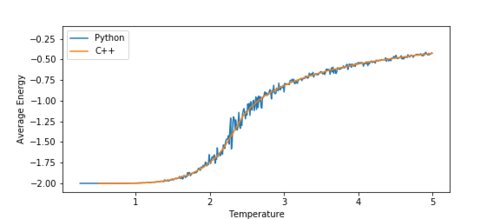
  Figure 13a Average Energy
• 
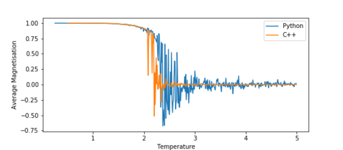
  Figure 13b Average Magnetisation
• 
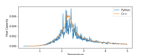
  Figure 13c Heat Capacity

At a first glance, we can see that they have a lot of similarities. The average energy graph (figure 13a) fits perfectly with the C++ data. The magnetisation (figure 13b), however, fluctuates significantly more than the C++ data. This is most likely due to shorter runtimes for the python simulation. The shorter the runtime, the more fluctuations will be visible in the critical region.

The heat capacity (figure 13c) also fits fairly well with the C++ data. Even with the shorter runtimes, the curve still follows the shape of the C++ data. The height of the peak, however, does not fit well - this can also be attributed to shorter runtimes and the fluctuations in the system. The peak, however, still occurs at the same temperature, which is important, as we want to use this data to calculate the Curie temperature for an infinite lattice.

TASK: Write a script to read the data from a particular file, and plot C vs T, as well as a fitted polynomial. Try changing the degree of the polynomial to improve the fit — in general, it might be difficult to get a good fit! Attach a PNG of an example fit to your report.

A python function was written to read a file containing the data for one of the simulation, extract it, and plot it alongside a fitted polynomial.

def plot_and_fit(FILE, degree):
"Extracts the Heat Capacity data from a file and plots it against a polynomial fit"
    data=loadtxt(FILE)
    T=data[:,0]
    E=data[:,1]
    E2=data[:,2]
    var=E2-E**2
    C=C_v(var, T)
    fit=np.polyfit(T,C,degree)
    T_min = np.min(T)
    T_max = np.max(T)
    T_range = np.linspace(T_min, T_max, 1000)
    fitted_C_values = np.polyval(fit, T_range)
    plot(T,C, linestyle=none, marker='o', markersize=1)
    plot(T_range, fitted_C_values)
    xlabel('Temperature')
    ylabel('Heat Capacity')
    show()

By varying the degree of the fitted polynomial, it was easily possible to improve the fit. Figures 14 and 15 show how the fit improves as the degree of the fitted polynomial increases. If the .gif files do not show, click on the thumbnails to view.

• 
  Figure 14 Heat Capacity vs Temperature for a 2x2 lattice. Once the polynomial reaches a degree of 10 the fit does not improve.
• 
  Figure 15 Heat Capacity vs Temperature for an 8x8 lattice. Once the polynomial reaches a degree of 20 the fit does not improve much.

TASK: Modify your script from the previous section. You should still plot the whole temperature range, but fit the polynomial only to the peak of the heat capacity! You should find it easier to get a good fit when restricted to this region.

The following function reads a file containing data for a simulation, extract the heat capacity, and fit a polynomial to the peak in the heat capacity. The region of the graph for which the polynomial fits against is determined by the variables Tmin and Tmax Therefore, if Tmin and Tmax are fitted against the peak, a much more accurate value for the coordinates of the peak can be obtained.

def peak_fit(FILE, degree, Tmin, Tmax):
    "Plots the heat capacity against a polynomial fit about the peak"
    data=loadtxt(FILE)
    T=data[:,0]
    E=data[:,1]
    E2=data[:,2]
    var=E2-E**2
    C=C_v(var, T)
    selection = np.logical_and(T>Tmin, T<Tmax)
    peak_T_values=T[selection]
    peak_C_values=C[selection]
    fit=np.polyfit(peak_T_values,peak_C_values,degree)
    T_range = np.linspace(np.min(T), np.max(T), 1000)
    fitted_C_values = np.polyval(fit, T_range)
    figure=figsize(8,4)
    plot(T,C, linestyle=none, marker='o', markersize=1)
    plot(T_range, fitted_C_values, label='Fitted Polynomial')
    xlabel('Temperature')
    ylabel('Heat Capacity')
    legend()
    title('Degree of Fitted Polynomial = '+str(degree))
    show()

Some additional lines were added to the above code to label and mark the graphs with lines to show the position of the peak.

• 
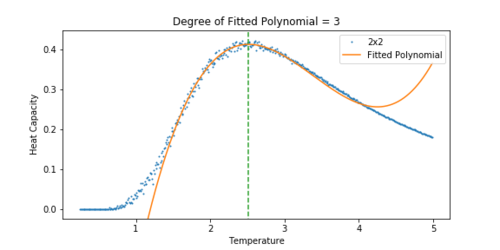
  Figure 16 Heat Capacity vs Temperature for a 2x2 lattice.
• 
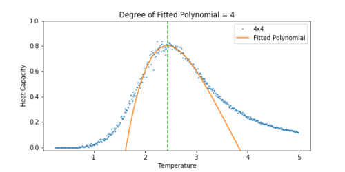
  Figure 17 Heat Capacity vs Temperature for a 4x4 lattice.
• 
  Figure 18 Heat Capacity vs Temperature for a 8x8 lattice.
• 
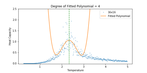
  Figure 19 Heat Capacity vs Temperature for a 16x16 lattice.
• 
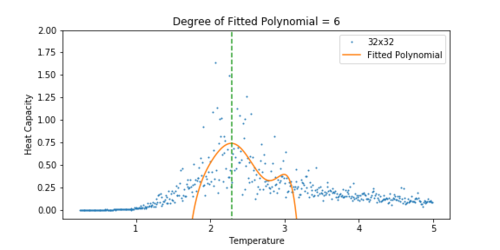
  Figure 20 Heat Capacity vs Temperature for a 32x32 lattice.

The heat capacity was easier to fit for a smaller lattice. As the lattice grew larger, the peak became significantly noisier, and so it was difficult to fit a polynomial to the peak. For the 32x32 lattice, a polynomial was chosen that approximately lined up with the peak. A dashed line has been added to all the plots to show how the peak of the fit corresponds to the peak in the heat capacity.

TASK: Find the temperature at which the maximum in C occurs for each datafile that you were given. Make a text file containing two columns: the lattice side length (2,4,8, etc.), and the temperature at which C is a maximum. This is your estimate of $T_C$ for that side length. Make a plot that uses the scaling relation given above to determine $T_{C,\mathrm{\infty }}$. By doing a little research online, you should be able to find the theoretical exact Curie temperature for the infinite 2D Ising lattice. How does your value compare to this? Are you surprised by how good/bad the agreement is? Attach a PNG of this final graph to your report, and discuss briefly what you think the major sources of error are in your estimate.

To extract the Curie temperature from the data, the temperature at which the heat capacity is at a maximum must be found. Therefore, the following piece of code was added to the fitting function above:

Cmax=np.max(fitted_C_values)
print(T_range[fitted_C_values==Cmax])

This finds the maximum value of the heat capacity in the fit, and prints the temperature at which it occurs. The calculated Curie temperatures for different lattice sizes are shown in the table below:

Lattice Size	2	4	8	16	32
Curie Temperature $T_C$	2.51798798798799	2.437327327327329	2.3566666666666687	2.3281981981982	2.285495495495497

From [15], if $1/L$ is plotted against $T_{C,L}$ there should be a straight line. By plotting this data and fitting the line as in figures 21 & 22, it is possible to find $T_{C,\mathrm{\infty }}$

• 
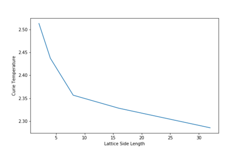
  Figure 21 A plot of Lattice Size vs. Curie Temperature, showing the inverse nature of the relationship
• 
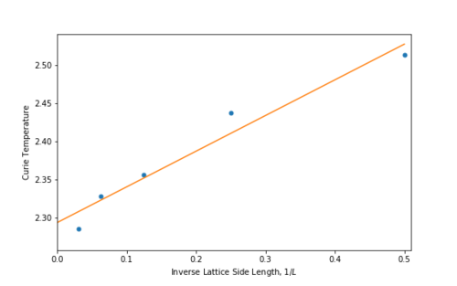
  Figure 22 A plot of $\frac{1}{L}$ vs Curie Temperature

From this fit, the Curie temperature for an infinite lattice is found to be:

$T_{C,\mathrm{\infty }}=2.292810310310312\pm 1.09\mathrm{\%}$

where the error is calculated taken from the covariance matrix from the numpy.polyfit() function. The analytical result found by Onsager in 1944 was:

$T_{C,\mathrm{\infty }}=\frac{2}{\ln (1+\sqrt{2})}=2.26918531421$

The percentage difference between the calculated and literature value is ~1.04%.

The main sources of error in calculating $T_{C,\mathrm{\infty }}$ are:

1. Problems with fitting polynomials to the peak - for the higher lattice sizes, it is difficult to get an accurate polynomial to fit the peak due to the amount of noise present. This creates variation in $T_{C,L}$, and therefore potential error in the value of $T_{C,\mathrm{\infty }}$.
2. The problems with noise in the heat capacity comes from not running the simulation for long enough to obtain a good average. The program written in C++ was able to be run with much longer runtimes, reducing the number of fluctuations close to the peak in the heat capacity.

Closing Remarks

The beauty of the Ising Model is its simplicity. By applying two simple rules to a lattice of spins (equations [1] and [7]), it is possible to observe a phase transition at the Curie Temperature. The model even shows effects of criticality close to the critical point. By applying some simple code to an array, it was possible to accurately model a complicated physical system, without the need for heavy computation of partition functions.