Rep:Ha3915cmp

Introduction to the Ising Model

TASK: Show that the lowest possible energy for the Ising model is $E = - D N J$ , where $D$ is the number of dimensions and $N$ is the total number of spins. What is the multiplicity of this state? Calculate its entropy.

The energy of the system in this model is only dependant on the interaction energies between adjacent spins in the lattice. This assumes that there is no external magnetic field applied to the system. The energy is given by:

E = - \frac{1}{2} J \sum_{i}^{N} \sum_{j \in n e i g h b o u r s (i)} s_{i} s_{j}

Hence, it can be seen that the minimum energy is achieved when all the spins are parallel, $J$ is a constant known as the exchange energy which is a result of Pauli's exclusion principle which states that electrons must not have the same set of quantum numbers. Therefore aligned spins cannot occupy the same state, thus electron repulsion is reduced and the total energy is minimised.^[1] ^[2]

To calculate the total number of interactions, each lattice site and its interactions with its neighbours must be considered. There are 2 neighbours for each lattice site in each dimension (2 in 1D, 4 in 2D, 6 in 3D etc.), hence the total number of neighbour interactions is $= 2 N D$

However each interaction is counted twice, so dividing by 2 the total number of interactions is $= 0.5 \times 2 N D = N D$ .

Since all the spins are parallel in the minimum energy state, each interaction is $- J$ .

Thus

E = - J \times N D = - D N J

The minimum energy lattice can be arranged in 2 ways (has 2 microstates), all spin up or all spin down, as such, the entropy is therefore:

$S = k_{B} \ln Ω = k_{B} \ln 2 = 9.57 \times 1 0^{- 24} J / K$

TASK: Imagine that the system is in the lowest energy configuration. To move to a different state, one of the spins must spontaneously change direction ("flip"). What is the change in energy if this happens ( $D = 3, N = 1000$ )? How much entropy does the system gain by doing so?

Energy of ground state with $D = 3, N = 1000$ is $- 3000 J$ with a single flipped spin, this becomes $3 \times (1 - 999) J = - 2994 J$ , a difference of $+ 6 J$ .

for entropy: $S = k_{B} \ln Ω = k_{B} \ln 2000 - k_{B} \ln 2 = k_{B} \ln 1000$

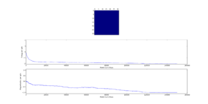
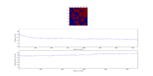
TASK: Calculate the magnetisation of the 1D and 2D lattices in figure 1. What magnetisation would you expect to observe for an Ising lattice with $D = 3, N = 1000$ at absolute zero?

1D lattice: magnetisation = +1

2D lattice: magnetisation = +1

At absolute zero, no entropic effects would be relevant and the system will be in the lowest energy state, with all spins parallel. Thus the magnetisation would be $\pm 1000$

Calculating the energy and magnetisation

TASK: complete the functions energy() and magnetisation(), which should return the energy of the lattice and the total magnetisation, respectively. In the energy() function you may assume that $J = 1.0$ at all times (in fact, we are working in reduced units in which $J = k_{B}$ , but there will be more information about this in later sections). Do not worry about the efficiency of the code at the moment — we will address the speed in a later part of the experiment.

    def energy(self):
        "Return the total energy of the current lattice configuration."
        #inpuy = array  [[1,1,1],
        #                [1,1,1],
        #                [1,1,1]]


        energy = 0.0
        N=self.n_rows
        M=self.n_cols
        for x in range(len(self.lattice)): #loops over rows
            for y in range(len(self.lattice)): #loops over columns
                currspin = self.lattice[x,y] # considering one spin at a time - current spin
                #summing the neighbours, if neighbour outside of lattice, return to 0th index of either rows or columns depending on 
                #which end of the lattice you're on.
                neighbours = self.lattice[(x+1)%N, y] + self.lattice[x,(y+1)%M] + self.lattice[(x-1)%N, y] + self.lattice[x,(y-1)%M]
                #multiply by neighbours
                energy += -neighbours*currspin
        return energy/2 #account for double counting.

    def magnetisation(self):
        "Return the total magnetisation of the current lattice configuration."
        magnetisation=np.sum(self.lattice) #sum all spins
        return magnetisation

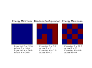
TASK: Run the ILcheck.py script from the IPython Qt console using the command

%run ILcheck.py

The displayed window has a series of control buttons in the bottom left, one of which will allow you to export the figure as a PNG image. Save an image of the ILcheck.py output, and include it in your report.

ILcheck.py checks the energy and magnetisation values obtained by the above code against known (expected) values for 3 lattices. It can be seen that all the numbers agree, therefore the code passed the test cases

Introduction to the Monte Carlo simulation

TASK: How many configurations are available to a system with 100 spins? To evaluate these expressions, we have to calculate the energy and magnetisation for each of these configurations, then perform the sum. Let's be very, very, generous, and say that we can analyse $1 \times 1 0^{9}$ configurations per second with our computer. How long will it take to evaluate a single value of ${⟨ M ⟩}_{T}$ ? For 100 spins, there are $2^{100}$ configurations. At $1 0^{9}$ configurations per second, it would take $1.27 \times 1 0^{21}$ seconds to finish the calculation = 40271435819381 years.

TASK: Implement a single cycle of the above algorithm in the montecarlocycle(T) function. This function should return the energy of your lattice and the magnetisation at the end of the cycle. You may assume that the energy returned by your energy() function is in units of $k_{B}$ ! Complete the statistics() function. This should return the following quantities whenever it is called: $< E >, < E^{2} >, < M >, < M^{2} >$ , and the number of Monte Carlo steps that have elapsed.

    def montecarlostep(self, T):
        # complete this function so that it performs a single Monte Carlo step
        energy0 = self.energy()#get init lattice energy
        #the following two lines will select the coordinates of the random spin for you
        random_i = np.random.choice(range(0, self.n_rows))
        random_j = np.random.choice(range(0, self.n_cols))
        self.lattice[random_i,random_j]= -1*self.lattice[random_i,random_j] #flip a random spin
        energy1=self.energy()#get new energy
        delE= energy1-energy0# diffience between new and init energy
        if delE <0: #if difference < 0
            pass #accept new config
        if delE>0:#if difference > 0
            random_number = np.random.random()
            if float(random_number) <= np.exp(-1*(delE/T)):# compare random number [0,1) with boltzmann distribution
                pass #accept new config
            if float(random_number) >= np.exp(-1*(delE/T)):
                self.lattice[random_i,random_j]=-1*self.lattice[random_i,random_j]#reject new config, revert to old one
        self.n_cycles+=1
        self.E+=self.energy()
        self.E2+= (self.energy())**2 
        self.M+= self.magnetisation()
        self.M2+= (self.magnetisation())**2
    
        return self.energy(),self.magnetisation() 
        
                

    def statistics(self):
        # complete this function so that it calculates the correct values for the averages of E, E*E (E2), M, M*M (M2), and returns them
        return self.E/(self.n_cycles),self.E2/(self.n_cycles),self.M/(self.n_cycles),self.M2/(self.n_cycles),self.n_cycles

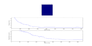
TASK: If $T < T_{C}$ , do you expect a spontaneous magnetisation (i.e. do you expect $⟨ M ⟩ \neq 0$ )? When the state of the simulation appears to stop changing (when you have reached an equilibrium state), use the controls to export the output to PNG and attach this to your report. You should also include the output from your statistics() function.

The original ILanim.py was modified to accept 5 values from IsingLattice.statistics(), this was to increase compatibility of the code with the future iterations and other scripts.

    E, E2, M, M2, n_cyc = il.statistics()
    print("Averaged quantities:")
    print("E = ", E/spins)
    print("E*E = ", E2/spins/spins)
    print("M = ", M/spins)
    print("M*M = ", M2/spins/spins)

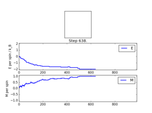
ILanim.py for an 8x8 lattice, at temperature = 0.5. This is below the critical temperature: the system converged to the minimum energy state, with all spins parallel. The energy exchange effect dominates over the entropic effects at this temperature.

This was the debug output:

Averaged quantities:
E =  -1.54994419643
E*E =  2.6142171224
M =  0.74767485119
M*M =  0.619416736421

Accelerating the code

TASK: Use the script ILtimetrial.py to record how long your current version of IsingLattice.py takes to perform 2000 Monte Carlo steps. This will vary, depending on what else the computer happens to be doing, so perform repeats and report the error in your average!

Trial	Time /s
1	6.1927
2	6.2243
3	6.2027
4	6.1729
5	6.1671

Average = 6.191 $\pm$ 0.024 seconds

TASK: Look at the documentation for the NumPy sum function. You should be able to modify your magnetisation() function so that it uses this to evaluate M. The energy is a little trickier. Familiarise yourself with the NumPy roll and multiply functions, and use these to replace your energy double loop (you will need to call roll and multiply twice!).

    def energy(self):
        "Return the total energy of the current lattice configuration."
        #inpuy = array  [[1,1,1],
        #                [1,1,1],
        #                [1,1,1]]
        energy = 0.0
        N=self.n_rows
        M=self.n_cols
        # Roll the lattice vertically and multiply with original to find total vertical interactions
        # Roll the lattice horizontally and multiply with original to find total horizontal interactions
        # sum the interactions
        return -np.sum(np.multiply(self.lattice,np.roll(self.lattice,-1,axis=0)) + np.multiply(self.lattice,np.roll(self.lattice,-1,axis=1)))


    def magnetisation(self):
        "Return the total magnetisation of the current lattice configuration."
        magnetisation=np.sum(self.lattice)
        return magnetisation

TASK: Use the script ILtimetrial.py to record how long your new version of IsingLattice.py takes to perform 2000 Monte Carlo steps. This will vary, depending on what else the computer happens to be doing, so perform repeats and report the error in your average!

Trial	Time /s
1	0.4913
2	0.5374
3	0.5304
4	0.5703
5	0.4932

Average = 0.525 $\pm$ 0.033 seconds

The effect of temperature

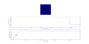
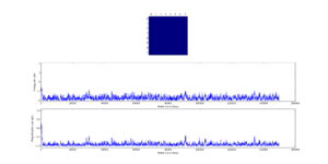
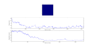
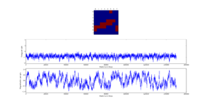
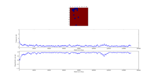
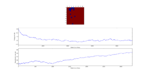
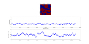
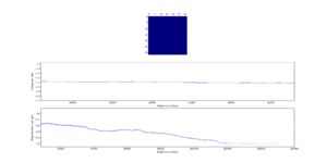
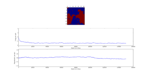
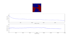
TASK: The script ILfinalframe.py runs for a given number of cycles at a given temperature, then plots a depiction of the final lattice state as well as graphs of the energy and magnetisation as a function of cycle number. This is much quicker than animating every frame! Experiment with different temperature and lattice sizes. How many cycles are typically needed for the system to go from its random starting position to the equilibrium state? Modify your statistics() and montecarlostep() functions so that the first N cycles of the simulation are ignored when calculating the averages. You should state in your report what period you chose to ignore, and include graphs from ILfinalframe.py to illustrate your motivation in choosing this figure.

Lattice size	Temperature	Equilibrium steps
6x6	1	~300
8x8	1	~900
8x8	2	~2500
8x8	3	doesn't reach equilibrium as above critical temperature, entropically driven spin flipping.
16x16	1	~4000
16x16	2	doesn't reach minimum energy, finds local minima and remains in metastable state
16x16	3	doesn't reach equilibrium as above critical temperature, entropically driven spin flipping.
32x32	1	~12000
32x32	2	doesn't reach minimum energy, finds local minima and remains in metastable state
32x32	3	doesn't reach equilibrium as above critical temperature, entropically driven spin flipping.

It can be seen that the number of steps required for the system to converge to the final state increases with lattice size. Below the critical temperature (which was ~3 for most lattice sizes tested), it is expected that all spins should be the same, hence achieving the minimum energy configuration. It takes longer for larger lattices to converge, since we selected random spins to flip thus, there is a greater probability of selecting the 'wrong' spin. For the smaller lattices, the system converges within a few hundred steps.Thermal energy can help with the spin flipping and therefore temperature is a factor to consider, the higher the temperature the more rapid the flipping. Approaching the critical temperature, more fluctuations are possible, and more steps are required for the system to minimise the energy. Above the critical temperature, entropic effects dominate.

With larger lattices, the minimum energy configuration is not always found, this is because the system lies in a metastable state where there are regions of aligned spins within the system but not all spins are aligned. This is a local minimum on the potential energy surface and the global minimum is not found.

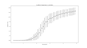
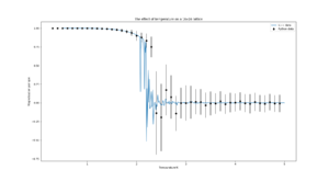
TASK: Use ILtemperaturerange.py to plot the average energy and magnetisation for each temperature, with error bars, for an $8 \times 8$ lattice. Use your initution and results from the script ILfinalframe.py to estimate how many cycles each simulation should be. The temperature range 0.25 to 5.0 is sufficient. Use as many temperature points as you feel necessary to illustrate the trend, but do not use a temperature spacing larger than 0.5. T NumPy function savetxt() stores your array of output data on disk — you will need it later. Save the file as 8x8.dat so that you know which lattice size it came from.

Energy	Magnetisation

This simulation ran for 250000 steps for the temperature range 0.3 to 5.0 with a temperature step of 0.1. Each simulation was run 5 times and the mean is plotted with error bars.

The code was modified to correct the average such that the first ncols x nrows x 200 steps were discarded whilst the system equilibrated, thus giving a more accurate average.

        if self.n_cycles >= self.n_rows*self.n_cols*200:
            self.E+=self.energy()
            self.E2+= (self.energy())**2 
            self.M+= self.magnetisation()
            self.M2+= (self.magnetisation())**2
    
        return self.energy(),self.magnetisation() 
        
                

    def statistics(self):
        # complete this function so that it calculates the correct values for the averages of E, E*E (E2), M, M*M (M2), and returns them
        cyc=self.n_cycles-(self.n_rows*self.n_cols*200)
        return self.E/(cyc),self.E2/(cyc),self.M/(cyc),self.M2/(cyc),self.n_cycles

The effect of system size

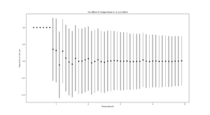
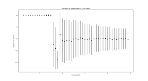
TASK: Repeat the final task of the previous section for the following lattice sizes: 2x2, 4x4, 8x8, 16x16, 32x32. Make sure that you name each datafile that your produce after the corresponding lattice size! Write a Python script to make a plot showing the energy per spin versus temperature for each of your lattice sizes. Hint: the NumPy loadtxt function is the reverse of the savetxt function, and can be used to read your previously saved files into the script. Repeat this for the magnetisation. As before, use the plot controls to save your a PNG image of your plot and attach this to the report. How big a lattice do you think is big enough to capture the long range fluctuations?

Lattice size	Energy	Magnetisation
2x2
4x4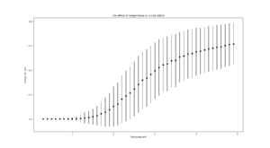
8x8
16x16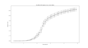
32x32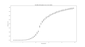

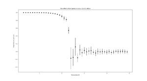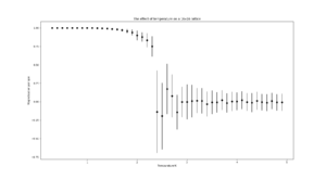
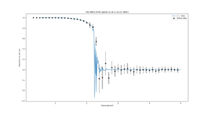
It should be noted that for all lattice sizes, the error bar sizes increase with temperature. At low temperatures, below the critical temperature, their sizes are negligible, as we get closer and closer to the critical temperature(~2-3 depending on lattice size), more states are accessible by the system so there's greater variation until they reach a maximum at the critical temperature.

As the lattice size increases, the overall size of the bars decrease as the variation in energy from spin flips is much smaller relatively.

16x16 and larger lattice sizes are big enough to capture long-range fluctuations as a spin flip causes a more subtle change in the system's energy.

Determining the heat capacity

TASK: By definition,

$C = \frac{\partial ⟨ E ⟩}{\partial T}$

From this, show that

$C = \frac{V a r [E]}{k_{B} T^{2}}$

(Where $V a r [E]$ is the variance in $E$ .)

$q = \sum_{i} e^{- β ε_{i}}$ , where $β = \frac{1}{k_{B} T}$ and $ε_{i}$ is the energy of each state $i$ ^[3]:

⟨ E ⟩ = \frac{E}{N} = \frac{1}{N} \sum N_{i} ε_{i} = \frac{1}{q} \sum ε_{i} \exp (- β ε_{i}) = - \frac{1}{q} \frac{\partial q}{\partial β} = - \frac{\partial \ln q}{\partial β}

⟨ E^{2} ⟩ = \frac{1}{q} \frac{\partial^{2} q}{\partial β^{2}}

V a r [E] = ⟨ E^{2} ⟩ - ⟨ E ⟩^{2}

C_{V} = \frac{\partial ⟨ E ⟩}{\partial T}

V a r [E] = \frac{1}{q} \frac{\partial^{2} q}{\partial β^{2}} - {(- \frac{1}{q} \frac{\partial q}{\partial β})}^{2}

= \frac{\partial}{\partial β} (\frac{1}{q} \frac{\partial q}{\partial β})

Hence:

V a r [E] = \frac{\partial}{\partial β} (\frac{1}{q} \frac{\partial q}{\partial β}) = \frac{\partial^{2} \ln q}{\partial β^{2}}

since $⟨ E ⟩ = - \frac{\partial \ln q}{\partial β}$ , and $\frac{\partial}{\partial β} = - k_{B} T^{2} \frac{\partial}{\partial T}$

V a r [E] = \frac{\partial^{2} \ln q}{\partial β^{2}} = - \frac{\partial}{\partial β} (- \frac{\partial \ln q}{\partial β}) = - \frac{\partial}{\partial β} ⟨ E ⟩ = - (- k_{B} T^{2} \frac{\partial}{\partial T}) ⟨ E ⟩ = k_{B} T^{2} C_{V}

Hence:

C_{V} = \frac{V a r [E]}{k_{B} T^{2}}

TASK: Write a Python script to make a plot showing the heat capacity versus temperature for each of your lattice sizes from the previous section. You may need to do some research to recall the connection between the variance of a variable, $V a r [X]$ , the mean of its square $⟨ X^{2} ⟩$ , and its squared mean ${⟨ X ⟩}^{2}$ . You may find that the data around the peak is very noisy — this is normal, and is a result of being in the critical region. As before, use the plot controls to save your a PNG image of your plot and attach this to the report.

Lattice size	Heat Capacity plot
2x2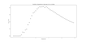
4x4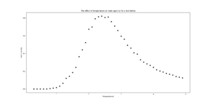
8x8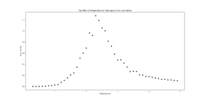
16x16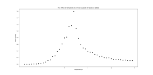
32x32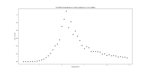
All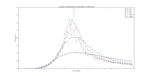

Locating the Curie temperature

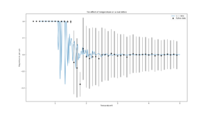
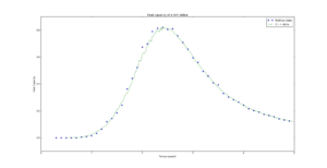
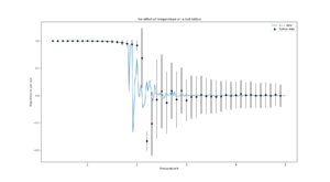
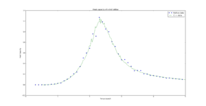
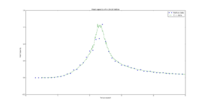
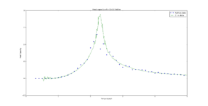
TASK: A C++ program has been used to run some much longer simulations than would be possible on the college computers in Python. You can view its source code here if you are interested. Each file contains six columns: $T, E, E^{2}, M, M^{2}, C$ (the final five quantities are per spin), and you can read them with the NumPy loadtxt function as before. For each lattice size, plot the C++ data against your data. For one lattice size, save a PNG of this comparison and add it to your report — add a legend to the graph to label which is which. To do this, you will need to pass the label="..." keyword to the plot function, then call the legend() function of the axis object (documentation here).

Lattice size	Energy	Magnetisation	Heat Capacity
2x2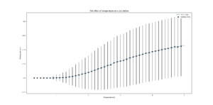
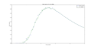4x4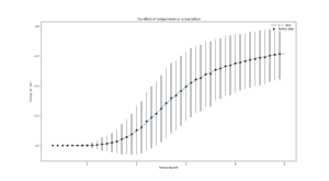
8x8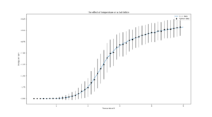
16x16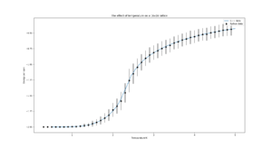
32x32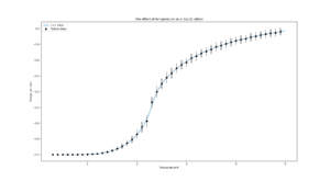

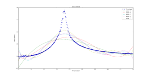
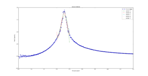
TASK: write a script to read the data from a particular file, and plot C vs T, as well as a fitted polynomial. Try changing the degree of the polynomial to improve the fit — in general, it might be difficult to get a good fit! Attach a PNG of an example fit to your report.

TASK: Modify your script from the previous section. You should still plot the whole temperature range, but fit the polynomial only to the peak of the heat capacity! You should find it easier to get a good fit when restricted to this region.

Polyfit orders	Polyfit reduced range	Polyfit reduced range zoom

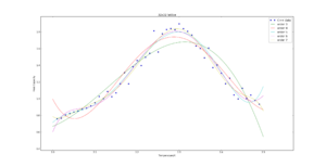The polynomial order used for the next tasks is 8.

TASK: find the temperature at which the maximum in C occurs for each datafile that you were given. Make a text file containing two colums: the lattice side length (2,4,8, etc.), and the temperature at which C is a maximum. This is your estimate of $T_{C}$ for that side length. Make a plot that uses the scaling relation given above to determine $T_{C, \infty}$ . By doing a little research online, you should be able to find the theoretical exact Curie temperature for the infinite 2D Ising lattice. How does your value compare to this? Are you surprised by how good/bad the agreement is? Attach a PNG of this final graph to your report, and discuss briefly what you think the major sources of error are in your estimate.

T_{C, L} = \frac{A}{L} + T_{C, \infty}

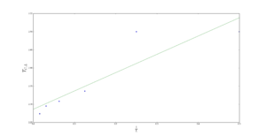
The plot of $T_{C, L}$ against $\frac{1}{L}$ gives a straight line, with intercept $T_{C, \infty}$ and gradient $A$ Fitting the C++ data gives $T_{C, \infty} = 2.28 \pm 0.0174 \frac{J}{k_{B}}$ which is only slightly off the theorectical reference value^[1] of $T_{C, \infty} \approx 2.269 \frac{J}{k_{B}}$ . This is a great result considering the sampling method used and the approximations made. The main source of error is the linear regression error, which is almost a 1% error. Other errors include fitting the peaks in each heat capacity plot, finding the max temperature and problems with the simulations themselves such as the system not reaching equilibrium or staying in the metastable state.

References

↑ ^1.0 ^1.1 B. Liu, M. Gitterman, American Journal of Physics, 71, 806 (2003), pp. 1-4
↑ R. Fitzpatrick, 2006, The Ising Model, Computational Physics, accessed from http://farside.ph.utexas.edu/teaching/329/lectures/node110.html on 22 November 2017.
↑ P. Atkins and J. de Paula, Atkins' Physical Chemistry, Oxford University Press, UK, 8th edn, 2006, pp. 564-573

[:0-1] 1.0 ^1.1 B. Liu, M. Gitterman, American Journal of Physics, 71, 806 (2003), pp. 1-4

[2] R. Fitzpatrick, 2006, The Ising Model, Computational Physics, accessed from http://farside.ph.utexas.edu/teaching/329/lectures/node110.html on 22 November 2017.

[3] P. Atkins and J. de Paula, Atkins' Physical Chemistry, Oxford University Press, UK, 8th edn, 2006, pp. 564-573

[1]

[2]

[3]