Rep:Gm1110LiquidSim
overall: you show a basic understanding of the sciece here but your writing style needs a bit of work before you write your thesis - you need to be punchier with your conclusions and take home messages. Think about the underlying science, find an intersting application/hot topic and write punchy. You haven't really elaborated on what you expect for the heat capacity also you show a lack of understanding with regard to a Lennard-Jones fluid describing rotational and vibrational DoFs. These are point particles modelled under a 12-6 LJ forcefield - they move but don't vibrate or rotate. Needs a bit of work... Mark: 60/100.
Abstract
The science in this lab calculated equation of state, heat capacity and the diffusion coefficient from two methods - msd and VACF. Unless you have generated a new technique, someone reading your report won't care that you've tested different timesteps etc. The "radial distribution functions calculated confirmed that the simulation were producing structurally accurate systems for solid, liquid and vapour" - again I expect you as the scientist to tell me what you have is solid, liquid and vapour. Then you, as the scientist, should compare them and comment on them - this isn't a critical comment. Putting your data in the abstract is good but here you don't state your ultimate conclusion (if you had one) - are either of these methods for measuring D better? Overall, you need to work on your abstract writing. Keep it short and sweet, think critically for the reader (the reader should read your report to think for themselves! Give them a taster) and target take home messages.
Preliminary tests were conducted to determine a suitable timestep value for simulations into a Lennard-Jones fluid (0.0025 s). It was shown that the density of the systems decreased with an increase in temperature, and that running the simulations at higher pressures led to a greater deviation from ideality. A further investigation into heat capacity showed that ease of heating increases as temperature increases, and that heat capacity decreases for lower density systems.
The radial distribution functions calculated confirmed that the simulations were producing structurally accurate systems for solid, liquid and vapour phases, allowing for calculation of the diffusion coefficients via the mean square displacement method and the velocity autocorrelation function.
For the more accurate 1,000,000 atom simulation, the diffusion coefficients were calculated to be -6.83x10⁻⁶, 0.0698 and 2.47 m2 s-1 for the solid, liquid and vapour phases respectively using the mean square displacement method, and 4.55x10⁻⁵, 0.0901 and 3.27 m2 s-1 using the velocity autocorrelation function.
Introduction
I've seen the perfume used as a example here way too many times and I know who originally came up with the idea. Not a particularly strong intro... You need to perform a literature review - have there been experiments on this? It's also a really short intro.
The process of diffusion is important in all aspects of life, from the perfume industry[1] to insulation[2]. For example, fragrance companies may need to know how long their perfume will last before it completely diffuses away after application, or the way in which the different components of their fragrance interact. In the case of insulation, investigating how thermal energy diffuses through different materials is very important for improving their efficiencies. Computer simulations are often used nowadays to predict the time taken for certain processes to occur, and the mechanisms that drive them, and these results can used as a preliminary basis to conduct physical experiments.
Aims and Objectives
In your thesis, you can bullet point your aims and objectives.
The main aim of the experiment was to determine the diffusion coefficient for the solid, liquid and vapour phases of a Lennard-Jones fluid using both the mean squared displacement method and velocity autocorrelation function method. and compare them.
In order to achieve this, it was first necessary to determine an appropriate timestep with which to run simulations, and investigate the effect of temperature and pressure on the density of the system. Other aims included seeing how heat capacity varied as a function of temperature for different densities, and calculating the radial distribution function for the three phases from simulations using VMD. If you mention you use software, MUST cite it...
Methods
Not a bad methods section - sticking to the style model-forcefield-tools.
All simulations of the Lennard-Jones fluid were run using the LAMMPS software, and all quantities used were in reduced units.
Part 1: Investigation into Simulation Timestep in the NVE Ensemble
A simulation box consisting of 10 x 10 x 10 unit cells of a simple cubic lattice with an atomic density of 0.8 was defined. The atomic mass was set to 1.0 and the Lennard-Jones pairwise interaction cutoff distance was set to 3.0. The pairwise forcefield coefficients ε (potential well depth) and σ (zero-potential distance) were both set to 1.0. Five simulations were run for differing timestep values (0.0010, 0.0025, 0.0075, 0.0100 and 0.0150).
Part 2: Equations of State in the NpT Ensemble
The simulation box was increased to consist of 15 x 15 x 15 unit cells of the same simple cubic lattice defined in part 1. A total of ten simulations were run in the NpT ensemble, varying temperature (2.0, 4.0, 6.0, 8.0 and 10.0) at two different densities (1.8 and 2.8) using the timestep value of 0.0025 determined in Part 1.
Part 3: Calculation of Heat Capacity
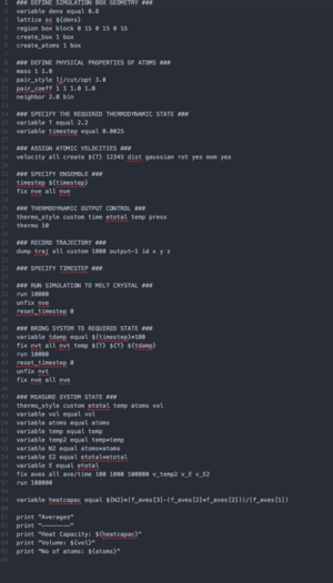
The simulation box from Part 2 was used, with the density altered to take the values 0.2 and 0.8. Five simulations were run for each, with varying values of temperature (2.0, 2.2, 2.4, 2.6 and 2.8). A copy of the script written for this simulation can be found by clicking the image below:
Part 4: Radial Distribution Functions
The simulation boxes used previously were altered to take a timestep of 0.002 and a L-J cutoff distance of 3.2, after which the solid, liquid and vapour phases were defined as having (density, temperature) values of (1.2, 1.2), (0.8, 1.2) and (0.05, 1.1) respectively[3]. In particular, the solid phase was defined as having a face-centred cubic lattice, instead of the simple cubic lattice used for the liquid and vapour phases. VMD was used to analyse the trajectories for the three phases, with the distance between points in the generated RDF set to 0.05.
Part 5: Diffusion Coefficient
The results from Part 4 were used to graph the mean squared displacement as a function of time, after which the gradient of the linear portion of the graph was extracted and used to calculate the diffusion coefficient from the equation:

The diffusion coefficients were also calculated from the velocity autocorrelation function from the equation:

where ![]() is the velocity autocorrelation function.
is the velocity autocorrelation function.
Results and Discussion
Investigation into Simulation Timestep in the NVE Ensemble
tick
Simulations were run using the five different timesteps 0.0010, 0.0025, 0.0075, 0.0100 and 0.0150, and a plot of the results can be seen below (Figure 1).

It was observed that the simulation run with a timestep of 0.0150 did not equilibrate. This was thought to have potentially been due to the timestep being too large, and therefore the simulation was missing too much detail to accurately simulate the fluid. The simulations run for timesteps of 0.0100 and 0.0075 did equilibrate (supporting the previous hypothesis that the 0.0150 timestep was too large), but converged at the wrong energy (approximately -3.181 and -3.183 respectively), indicating that the timesteps were still not quite small enough.
The final two simulations run at timesteps of 0.0025 and 0.0010 both equilibrated to the same, correct energy (approximately -3.184), indicating that both would be suitable for use in further simulations. It is preferable, however, to maximise the timestep when running simulations as a smaller timestep requires more data points, and is therefore more “expensive” and takes longer to run for no real added value. Hence it was decided that a timestep of 0.0025 would be suitable for running further simulations.
Equations of State in the NpT Ensemble
In your abstract you mentioned that the densities were different with pressure - where's your comment on this here? Also, should notice at high T a tendency to ideality - why?
Although specific values for temperature and pressure are specified for the simulations, in reality, the temperature and pressure of a system fluctuates over time and may therefore deviate away from the inputted values. Hence, the simulation calculates the pressure of the system at the end of every timestep, and adjusts the size of the simulation box such that the pressure once again corresponds to the specified value. Pressure controlled simulations are thus in the NpT ensemble and so volume (and therefore density) is not constant.
A total of ten simulations were run, and the resulting densities were plotted against temperature, along with values predicted by the ideal gas law and can be seen below (Figure 2).

Clearly, the simulated densities are lower than those predicted by the ideal gas law, and the discrepancy increases with increasing pressure. This is due to the fact that the ideal gas law assumes perfectly elastic collisions between point particles, but in reality, intermolecular repulsive forces cause the simulated densities to be lower. In addition, an increase in pressure causes the molecules to be pushed closer together and increases both the number of collisions as well as the repulsive forces, leading to a greater deviation from ideality.
Calculation of Heat Capacity
Switching to the NVT ensemble, the heat capacity of the system can be determined by considering the magnitude of fluctuations in the system’s energy from its average equilibrium state from the equation:

A total of ten simulations were run, and the average heat capacities were plotted as a function of temperature (Figure 3).

Heat capacity is a measure of the amount of energy required to increase the temperature of a substance. It is clear that the heat capacity is lower, and therefore easier to heat, for lower density systems as the particles are more spaced apart. This means that they are able to gain thermal energy more easily as they have more room for increased vibrations without an increase of repulsive forces or collisions compared to a higher density system.there are no vibrations in this system... only generated velocities calculated by the Maxwell-Boltzmann distribution It was also noted that the heat capacity decreased with increasing temperature. This is due to the fact that at higher temperatures, the gap between energy levels decreases as the particles occupy higher energy states, thus making it easier for the particles to be promoted to higher energy levels.
It is also clear that heat capacity decreases with increasing temperature (ie it is easier to heat a hotter object). This is due to the fact that as temperature increases, more rotational and vibrational energy levels become thermally accessible, leading to a faster increase in internal energy and thus a lower heat capacity. do we have any rotational or vibrational DoF here????? No.
Radial Distribution Functions
Radial distribution functions (g(r)) were calculated for the solid, liquid and vapour phases (see Figure 4) to check that the simulations were correctly reproducing the structural features of each phase. RDFs are essentially probability distribution functions for the likelihood of finding a particle at a given distance r away from a reference particle, and also gives information on the coordination sphere of the reference particle. The integral of the RDF (Figure 5) is also useful as it gives information on the number of atoms found at a distance r.


For small r, all three phases have g(r) ~ 0, indicating an atomic density of zero as there exists a minimum distance at which atoms can approach each other. Also, g(r) tends to 1 for all three phases with increasing r, which represents the fact that the local density becomes equivalent to the mean density of the system as a whole[4].
The graph of the solid phase shows sharp oscillating peaks, indicating that the atoms are strongly confined to their positions in the crystalline lattice, and the high degree of ordering means that although the osciallations do tend to g(r) = 1 for large r, this occurs much more slowly than for the other two phases[5]. No dynamic avergaing The first peak corresponds to the atoms nearest neighbours (of which there are 12), and the second and third peak correspond to the second and third nearest neighbours respectively (of which there are 6 and 24).
The graph for the liquid phase shows broad, gently oscillating peaks that rapidly decay to g(r) = 1. As with the solid phase, the oscillations indicate some structure in the system whereby the atoms are loosely bound to their original positions, but the broader peaks indicate that they have much more freedom to move away from their positions. local order - solid has the highest, liquid has shorter range order and gas has none
The graph for the vapour phase shows a single peak at approximately r = 1, after which it quickly decays back to g(r) = 1. This shows that the structure has very little to no order, and the particles are free to move unbound to any specific position.
Diffusion Coefficient
The general trends displayed in Figures 6-8 are as expected: the simulation does eventually establish linear behaviour, with the gradients increasing exponentially going from the solid to vapour phases. It is well known that diffusion in the vapour phase occurs much more readily than in the liquid phase, and more readily in the liquid phase than solid phase, and given that the diffusion coefficient is linearly correlated to the gradient of the mean square displacement, it was expected that the gradients of the graphs would increase in this manner. It was noted that the linear region of the solid phase plot (Figure 6) was quite noisy, but it was thought that this may be due to the small simulation size of 1,000 atoms.
The results from the simulation with 1,000,000 atoms (Figures 9-11) support the observations made with the 1,000 atom simulation. The only noticeable improvement from the 1,000 atom simulation was the reduction in noise of the linear region of the solid phase (Figure 9), suggesting that the assumption made previously to consider the more noisy region in Figure 6 as linear was correct, and that increasing the sample size did indeed improve the smoothness and accuracy of the curve. would the mill atoms sim be more accurate?
The gradient for the linear region of the plots were determined and used to calculate the diffusion coefficients (see table below).
| Table 1. Diffusion Coefficients Calculated Using the Mean Square Displacement Method | |||
|---|---|---|---|
The results obtained are reasonable figures. In comparison with the 1,000,000 atom simulation, the values calculated for the diffusion coefficient with 1,000 atoms yielded a 9.7%, 1.4% and 8.0% error for the solid, liquid and vapour phases respectively. This suggests that for systems involving atoms that are at either extreme with regards to their range of motion, a larger atomic sample size would be suitable for simulations, whereas for liquids, more time-efficient simulations can be accurately conducted using the smaller 1,000 atom sample size.
The positive values obtained for the liquid and vapour phase show that the atoms diffuse away from their original positions over time, whereas the negative value obtained for the solid phase arises as a consequence of attractive nearest neighbour interactions within the lattice structure[6]. sources of error?
The diffusion coefficient was also calculated using the velocity autocorrelation function (henceforth VACF).
| Table 2. Diffusion Coefficients Calculated Using the Velocity Autocorrelation Function | |||
|---|---|---|---|
Generally, the results show that the diffusion coefficients calculated using the VACF method and MSD method are both to the same order of magnitude, although the coefficients calculated via the VACF were 29-32% greater for the liquid and vapour phases.
The largest source of error in estimating the diffusion coefficient using the VACF was the number of atoms used in the simulations. This can be seen more clearly in Figures 16 and 17 which compare the VACF calculated for the liquid and vapour phases. The 1,000 atom simulation is clearly more noisy than the 1,000,000 atom simulation, indicating that the 1,000,000 atom simulation increases the reliability and accuracy of the results.What is the vacf? What does it show? How is the calculation of diff coeff inherently different using either method?
Conclusion
You've made a few conclusions in your R&D that you haven't shown here... This needs to be punchy and connect but with your original intro.. in your case, how does this mean good perfume?
A suitable timestep with which to run the simulations was determined to be 0.0025 s. Simulations then showed that the density of the systems decreased with an increase in temperature, and that running the simulations at higher pressures led to a greater deviation from ideality. A further investigation into heat capacity showed that ease of heating increases as temperature increases, and that heat capacity decreases for lower density systems. is this what you expect? Think about internal energy?
The radial distribution functions calculated show that the simulations were producing structurally accurate systems for the solid, liquid and vapour phases, allowing for calculation of the diffusion coefficients via the mean square displacement method and the velocity autocorrelation function.
For a 1,000 atom simulation, the diffusion coefficients were calculated to be -6.17x10⁻⁶, 0.0688 and 2.27 m2 s-1 for the solid, liquid and vapour phases respectively using the mean square displacement method, and -1.84x10⁻⁴, 0.0783 and 3.06 m2 s-1 using the velocity autocorrelation function. It was discovered that depending on the method used, and the specific phase being considered, that 1,000 atoms was not a sufficiently large enough sample to accurately model the systems, so 1,000,000 atom simulations were conducted.
For a 1,000,000 atom simulation, the diffusion coefficients were calculated to be -6.83x10⁻⁶, 0.0698 and 2.47 m2 s-1 for the solid, liquid and vapour phases respectively using the mean square displacement method, and 4.55x10⁻⁵, 0.0901 and 3.27 m2 s-1 using the velocity autocorrelation function. comparison?
Tasks
Correct, but some of your explanations in your report are not
Introduction to Molecular Dynamics Simulations
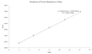
Task 1. For a default timestep value 0.1, estimate the positions of the maxima in the ERROR column as a function of time.
Task 2. What sort of a timestep do you need to use to ensure that the total energy does not change by more than 1% over the course of your "simulation"? Why do you think it is important to monitor the total energy of a physical system when modelling its behaviour numerically?
Using a timestep of 0.1990 meant that the total energy did not change by more than 1% over the course of the simulation (Figure 19). tick

The simulations are being run in isolated systems which requires total energy conservation, so large fluctuations in the energy would lead to inaccurate results.
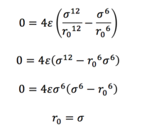
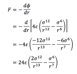
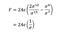
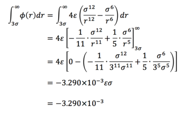
Task 3. For a single Lennard-Jones interaction, find the separation, r0, at which the potential energy is zero. What is the force at this separation? Find the equilibrium separation, req, and work out the well depth. Evaluate the integrals when σ = ε = 1.0.
(i) The Lennard-Jones interaction is given by:
Since r = r0 when ɸ = 0,
(ii) The force is given by
So at the separation r0 = σ,
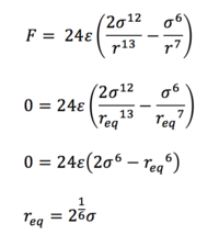
(iii) The equilibrium separation req occurs at the point at which all forces vanish, ie. when F = 0, so
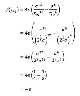
(iv) And the well depth is therefore given by
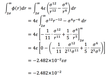
(v)
(vi)
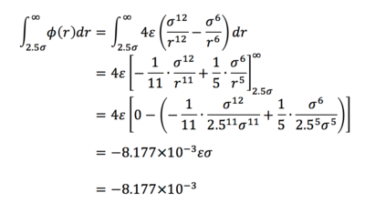
(vii)
tick
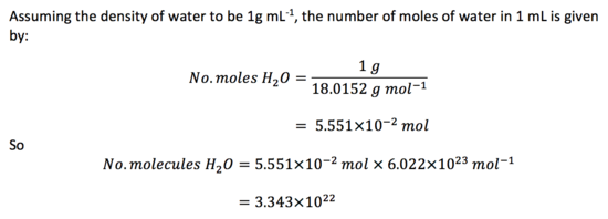
Task 4. Estimate the number of water molecules in 1ml of water under standard conditions. Estimate the volume of 10,000 water molecules under standard conditions.
For 10,000 water molecules,
Task 5. Consider an atom at position (0.5, 0.5, 0.5) in a cubic simulation box which runs from (0, 0, 0) to (1, 1, 1). In a single timestep, it moves along the vector (0.7, 0.6, 0.2). At what point does it end up, after the periodic boundary conditions have been applied?
After the timestep, the atom would be at position (0.5 + 0.7, 0.5 + 0.6, 0.5 + 0.2) = (1.2, 1.1, 0.7). Applying the boundary conditions, this is equivalent to the position (0.2, 0.1, 0.7).
Task 6. The Lennard-Jones parameters for argon are sigma = 0.34nm, ε/kB = 120K. If the LJ cutoff is r* = 3.2, what is it in real units? What is the well depth in kJ mol-1? What is the reduced temperature T* = 1.5 in real units?
(i)
(ii) It was previously determined in Task 1 that the well depth is - ε, so in real units,
(iii)
tick
Equilibration
Task 7. Why do you think giving atoms random starting coordinates causes problems in simulations?
If two atoms are generated too close to one another, then they would experience a large repulsive force, and would disrupt the behaviour of the surrounding atoms, causing the simulation to become inaccurate.
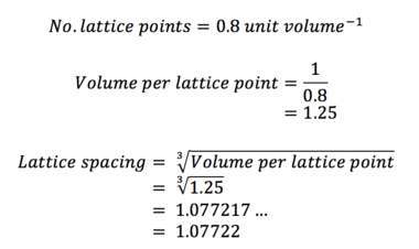
Task 8. Satisfy yourself that this lattice spacing corresponds to a number density of lattice points of 0.8. Consider instead a face-centred cubic lattice with a lattice point number density of 1.2. What is the side length of the cubic unit cell?
(i)
(ii) For a face-centred cubic lattice, note that the unit cell contains four atoms, as opposed to one atom with a simple cubic lattice. Then
Task 9. Consider again the face-centred cubic lattice from the previous task. How many atoms would be created by the create_atoms command if you had defined that lattice instead?
For a simple cubic lattice, there is 1 atom contained within each unit cell. However for face-centred cubic lattices, each unit cell contains 4 atoms so four times as many atoms are created than with the simple lattice (ie. 4000 atoms).
Task 10. Given that we are specifying xi (0) and vi (0), which integration algorithm are we going to use?
We will be using the Velocity-Verlet algorithm.
Task 11. In the code section "Specify Timestep", the second line (starting "variable timestep...") tells LAMMPS that if it encounters the text ${timestep} on a subsequent line, it should replace it by the value given. In this case, the value ${timestep} is always replaced by 0.001. In light of this, what do you think the purpose of these lines is? Why not just write "timestep 0.001 // run 100000"?
Defining the variable timestep allows us to reference the variable multiple times throughout the simulation if required, whilst preventing errors and making it easier to alter the code if we want to run the simulation for different timestep values.
Task 12. Make plots of energy, temperature, and pressure, against time for the 0.001 timestep experiment. Does the simulation reach equilibrium? How long does this take? Make a single plot of energy vs time for all of the timesteps. Of the five timesteps that you used, which is the largest to give acceptable results? Which one of the five is a particularly bad choice and why?
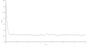
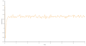
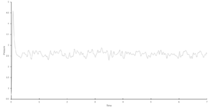
The 0.001 timestep experiment reaches equilibrium very quickly, within approximately 0.2s.
A single plot of energy vs time for all of the timesteps can be found in "Results & Discussion: Investigation into Simulation Timestep in the NVE Ensemble" (Figure 1), along with a detailed analysis, but in brief: the largest acceptable timestep is 0.0025, and a particularly bad choice would be 0.015 as it does not reach equilibrium.
Running Simulations under Specific Conditions
Task 13. We need to choose gamma so that the temperature is correct T=fancy T if we multiply every velocity by γ. Solve the following two equations to determine gamma:

Starting from the 2nd equation,
Task 14: Use the manual to find out the importance of the three numbers 100 1000 100000. How often will values of the temperature, etc., be sampled for the average? How many measurements contribute to the average? Looking to the following line ("run 100000"), how much time will you simulate?
Firstly, averages are taken for blocks of 100 values at a time to form the first set of averaged values (where av100,n is the average value for the nth block of 100 values). These values are then themselves averaged in blocks of 1000 values to form a second set of averaged values (av100,1 + av100,2 + ... + av100,1000)/1000 = av1000,1. Finally, these values are averaged once more in blocks of 100000 values.
The amount of time simulated can be found by multiplying the number of steps by the value of the timestep (eg. 100,000 steps of a 0.001 timestep simulates 100 seconds).
Task 15: Plot density as a function of temperature for both of the pressures that you simulated. Is your simulated density lower or higher? Justify this. Does the discrepancy increase or decrease with pressure?
See Figure 2 in "Results and Discussion: Equations of State in the NpT Ensemble" for the plot and subsequent discussion.
Heat Capacity Calculation
Task 16: Run simulations at densities of 0.2, 0.8 and temperatures of 2.0, 2.2, 2.4, 2.6, 2.8, plotting CV/V as a function of temperature, where V is the volume of the simulation cell, for both of your densities. Is the trend the one you would expect? Attach an example of one of your input scripts to your report.
For the plot of CV/V as a function of temperature, please see Figure 3 in "Results and Discussion: Calculation of Heat Capacity" and the subsequent discussion on why the trend was as expected. A copy of the input script can be found in "Method: Part 3: Calculation of Heat Capacity".
Structural Properties and the Radial Distribution Function
Task 17: Plot the RDFs for the three systems on the same axes. Discuss qualitatively the differences between the three RDFs, and what this tells you about the structure of the system in each phase. In the solid case, illustrate which lattice sites the first three peaks correspond to. What is the coordination number for each of the first three peaks?
See Figure 4 in "Results and Discussion: Radial Distribution Functions" for the plot and analysis.
Dynamical Properties and the Diffusion Coefficient
Task 18: Make a plot for each of your simulations, showing the mean squared displacement as a function of timestep. Are these as you would expect? Estimate D in each case. Repeat this procedure for the MSD data that you were given from the one million atom simulations.
See Figures 6-11 and Table 1 in "Results and Discussion: Diffusion Coefficient".
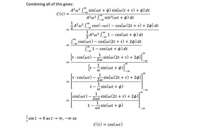
(Extension) Task 19: Evaluate the normalised velocity autocorrelation function for a 1D harmonic oscillator. On the same graph, with x range 0 to 500, plot C(τ) with Ω = 1/(2π) and the VACFs from your liquid and solid simulations. What do the minima in the VACFs for the liquid and solid system represent? Discuss the origin of the differences between the liquid and solid VACFs. Why is the harmonic oscillator VACF very different to the Lennard Jones solid and liquid?
See also "Results and Discussion: Diffusion Coefficient".
(Extension) Task 20: Use the trapezium rule to approximate the integral under the velocity autocorrelation function for the solid, liquid, and gas, and use these values to estimate D in each case. You should make a plot of the running integral in each case. Are they as you expect? Repeat this procedure for the VACF data that you were given from the one million atom simulations. What do you think is the largest source of error in your estimates of D from the VACF?
See "Results and Discussion: Diffusion Coefficient".
References
- ↑ http://onlinelibrary.wiley.com/doi/10.1002/aic.14106/epdf
- ↑ https://ac.els-cdn.com/S0142061513002032/1-s2.0-S0142061513002032-main.pdf?_tid=958b3390-1323-11e8-8822-00000aacb360&acdnat=1518790607_86d8f9f122450bef4ef7e3fc82f97936
- ↑ https://journals.aps.org/pr/pdf/10.1103/PhysRev.184.151
- ↑ Frenkel, Daan; Smit, Berend (2002). Understanding molecular simulation from algorithms to applications (2nd ed.). San Diego: Academic Press. ISBN 0122673514.
- ↑ https://en.wikibooks.org/wiki/Molecular_Simulation/Radial_Distribution_Functions
- ↑ https://journals.aps.org/prb/pdf/10.1103/PhysRevB.80.104203
