Rep:Ga714MD

General comments: This is a very nice report and you've understood the theory well. There is a bit of misunderstanding of the general principles of the correlation function but otherwise, very good. Mark: 80/100

Introduction

Molecular Dynamics simulations are pioneering the progress in the understanding of processes of biological macromolecules. Previous generations of simulations produced rather fixed structures of proteins. However, key to the function of a biological macromolecule are the conformational changes that it undergoes in contact with other molecules, particularly a target molecule. Thus, a more dynamics model, as simulated by Molecular Dynamics, gives a more refined model and a platform for improved research. Furthermore, variations of the Molecular Dynamics simulations allow for the study of protein folding, which could prove revolutionary in catalysis, and consequently industry.

Subsequently, an understanding of the simulation and constant evolution of this powerful tool are necessary in enhancing the classical approach to combat the weakness of Molecular Dynamics, namely its computational cost. In order to gain an accurate picture, large systems must be observed and it is the compromise between accuracy and computational cost that is delaying the progress in the field of biological macromolecules. This experiment aims to cover the fundamentals of the Molecular Dynamics simulation and highlight the strengths and weaknesses of the approximations.

Computational Methods

Molecular Dynamics treats the system under investigation classically, simply applying Newtonian mechanics as an approximation and allowing the particles in the system to interact. All the simulations were carried out using the Large-scale Atomic/Molecular Massively Parallel Simulator (LAMMPS). The LAMMPS simulations carried out incorporated the velocity-Verlet algorithm in order to integrate with respect to time the Newtonian equations of motion of the particles. This allows for the modelling of the particle interactions and computes their trajectories. Furthermore, there is a potential energy wall that causes nearby particle to repel preventing atoms collapsing into eachother and regions of abnormally high density. The input scripts were processed by the High Performance Computer at Imperial College London.

Introduction To Molecular Dynamics Simulation

The Harmonic Oscillator

In this exercise the velocity-Verlet algorithm was used to model the harmonic oscillator. The differences between the analytical solution to the harmonic oscillator and the velocity-Verlet computed model are analysed.

$x(t)=Acos(\omega t+\varphi )$ Eqn 1.

Eqn 1 shows the analytical solutions to the harmonic oscillator where the displacement from the equilibrium position varies with cos(time). Fig 1 shows the error in the velocity-Verlet modelled energy relative to the analytically-obtained energy. It can be seen that there is a cumulative character to the error as the maximum error appears to increase linearly with time. This indicates that the errors from each calculation compound, increasing the absolute error. The error fluctuates in a similar fashion to an absolute sinusoidal wave of increasing amplitude. The oscillating behaviour arises due to the overlapping trigonometric functions of the classical and the velocity-Verlet solutions to the energy. When the solutions are out of phase the error is at a maxima and, hence, when in phase the energy should be zero. However, the minima for the error appears to deviate from zero, this would indicate that with time the phase overlap of the two functions shifts slightly and so they do not overlap perfectly in-phase.

Fig 1. Plot of Absolute Error in Energy Vs Time with an Approximate Linear Function for the Error Maxima - 0.100 Timestep

The smaller the timestep the more accurate the Molecular Dynamics simulation. However, it also increases the computational cost and more calculations must be performed. Therefore, there exists a compromise between the accuracy of the simulation and time. For the closed system that is under investigation the total energy would be expected to remain constant, any potential energy would be converted to kinetic energy and vice-versa. However, Fig 2. demonstrates that this is not the case due to errors in the model. For the 0.100 timestep the deviations from the expected constant energy are extremely small. It is important to monitor the total energy of the system in order to understand the magnitude of the error. With increasing timestep this error would increase but would reduce the computational cost. The subsequent exercise involved attempting to find a reasonable timestep for the harmonic oscillator. It is determined that a 1% error is acceptable and therefore, the aim is to minimise the computational cost. From Fig 3 and Fig 4 it can be seen that the timestep that would result in a 1% maximum error in total energy would lie between these two. Given the approximations and assumptions of the Molecular Dynamics model, a 1% error is acceptable and a timestep less than 0.195 would simply invoke unnecessary computational cost. Correct

Fig 2. Plot of Energy Vs Time for 0.100 Timestep

Fig 3. Plot of Energy Vs Time for 0.195 Timestep

Fig 4. Plot of Energy Vs Time for 0.200 Timestep

Atomic Forces

Finding r₀

$\varphi \left(r\right)=4ϵ(\frac{{\sigma }^{12}}{r^{12}}-\frac{{\sigma }^6}{r^6})$

Potential Energy = 0

$0=4ϵ(\frac{{\sigma }^{12}}{r^{12}}-\frac{{\sigma }^6}{r^6})$

Discard 4$ϵ$ and rearrange

$\frac{{\sigma }^{12}}{r^{12}}=\frac{{\sigma }^6}{r^6}$

Multiply by $\frac{r^{12}}{{\sigma }^6}$

$r^6={\sigma }^6$

Take the positive sixth root of the equation to give r₀

$r_0=\sigma$Tick

Finding F at r₀

$F=-\frac{d\varphi (r)}{dr}$

So...

$F=-4ϵ\frac{d(\frac{{\sigma }^{12}}{r^{12}}-\frac{{\sigma }^6}{r^6})}{dr}$

Hence...

$F=-4ϵ(\frac{12{\sigma }^{12}}{r^{13}}-\frac{6{\sigma }^6}{r^7})$

At r₀ so substitute in r₀ = $\sigma$ and cancel

$F=-4ϵ((\frac{12}{\sigma }-\frac{6}{\sigma })$

Finally...

$F=\frac{24ϵ}{\sigma }$ when r = r₀ Tick

Finding r_eq

Equilibrium conditions met when resultant force is zero.

From before...

$F=-4ϵ(\frac{12{\sigma }^{12}}{r^{13}}-\frac{6{\sigma }^6}{r^7})$

F = 0, discard 4$ϵ$and rearrange

$\frac{12{\sigma }^{12}}{r_{eq}^{13}}=\frac{6{\sigma }^6}{r_{eq}^7}$

Multiply by $\frac{r_{eq}^{13}}{6{\sigma }^6}$

$r_{eq}^6=2{\sigma }^6$

Take the positive sixth root to give r_eq

$r_{eq}=\sigma \sqrt[6]{2}$ Tick

Finding the well depth

The well depth is the potential energy at the equilibrium interatomic distance.

From before...

$\varphi \left(r\right)=4ϵ(\frac{{\sigma }^{12}}{r^{12}}-\frac{{\sigma }^6}{r^6})$

r = r_eq and so substitute in $r_{eq}=\sigma \sqrt[6]{2}$

$\varphi (r_{eq})=4ϵ(\frac{{\sigma }^{12}}{(\sigma \sqrt[6]{2}{)}^{12}}-\frac{{\sigma }^6}{(\sigma \sqrt[6]{2}{)}^6})$

Simplify...

$\varphi (r_{eq})=4ϵ(\frac{1}{2^2}-\frac{1}{2})$

Evaluate...

$\varphi (r_{eq})=-ϵ$ Tick

Evaluating Integrals

Evaluate the following for n = 2.0, 2.5, 3.0

$\underset{n\sigma }{\overset{\mathrm{\infty }}{\int }}\varphi \left(r\right)\mathrm{d}r$

So...

$\underset{n\sigma }{\overset{\mathrm{\infty }}{\int }}4ϵ(\frac{{\sigma }^{12}}{r^{12}}-\frac{{\sigma }^6}{r^6})\mathrm{d}r$

Let $\sigma =ϵ=1$ and integrating gives...

$4{[\frac{1}{5r^5}-\frac{1}{11r^{11}}]}_n^{\mathrm{\infty }}$

Hence...

$4(\frac{1}{11n^{11}}-\frac{1}{5n^5})$

n	$\underset{n\sigma }{\overset{\mathrm{\infty }}{\int }}\varphi \left(r\right)\mathrm{d}r$
2.0	-0.02482 Tick
2.5	-0.00818 Tick
3.0	-0.00329 Tick

Periodic Boundary Conditions

Water Molecules in 1 mL

1 mL water = 1 g water

$n=\frac{m}{Mr}$

For 1 mL water

$n=\frac{1}{18.015}$

So...

$n=0.055509mol$

So number of water molecules

$n*N_A=3.34*10^{22}molecules$ Tick

Volume of 10000 Water Molecules Standard Conditions

$n=\frac{10000}{N_A}$

$m=18.015*\frac{10000}{N_A}$

$m=2.99*10^{-19}g$

At standard conditions 2.99 * 10^-19 g = 2.99 * 10^-19 mL Tick

Periodic Boundary Application

Atom start position (0.5, 0.5, 0.5)

Vector (0.7, 0.6, 0.2)

Atom final position (1.2, 1.1, 0.7)

Applying periodic boundary from (0, 0, 0) to (1, 1, 1)

Atom final position after periodic boundary application (0.2, 0.1, 0.7) Tick

Reduced Units

Real Unit Conversions for Argon

Converting reduced distance units

$r^{*}=\frac{r}{\sigma }$

$3.2=\frac{r}{0.34*10^{-9}}$

Hence...

$r=1.09*10^{-9}m$ Tick

Converting reduced energy units (well depth)

$\frac{ϵ}{K_B}=120$

So subbing in well depth....

$-ϵ=1.6567*10^{-21}Jperatom$

Unit conversion...

$ϵ=-1.6567*10^{-24}*N_{A}kJmo{l}^{-1}$

Finally...

$ϵ=-0.998kJmo{l}^{-1}$ Tick

Converting reduced temperature units

$T^{*}=\frac{K_{b}T}{ϵ}$

$1.5=\frac{120}{ϵ}$

Hence...

$T=180K$ Tick

Equilibrations

Issues With Randomly Designating Coordinate Positions

The issue with randomly assigning position coordinates is that with 1000 atoms to place in a finite box, it is extremely likely that two atoms will either be in extremely close proximity, or overlapping. The calculations account for a Lennard-Jones Potential to model the energy of particles with respect to inter-nuclear distance. On decreasing inter-nuclear separation below the equilibrium position the energy increases dramatically. This would have significant effects on the forthcoming simulation and introduce significant errors. Therefore, it is more accurate to place atoms on a lattice and allow them to equilibrate from these positions. and with higher energies, simulations require a smaller associated timestep

Number Density of Lattice and Unit Cell Length =

The side length of the cubic cell is 1.07722. Therefore, the volume of the cube is 1.25.

The equation for the number density is given by…

$\rho =\frac{N}{V}$

Subbing in values for simple cubic lattice V=1.25….

$\rho =\frac{1}{1.25}$

So…

$\rho =0.8$ Tick

For a lattice of number density 1.2, the unit cell length is given by…

$V=\frac{N}{\rho }$

Subbing values in 4 atoms per unit cell in FCC…

$V=\frac{4}{1.25}$

So…

$V=3.\dot{3}$

And therefore the cell length = 1.494. Tick

How Many Atoms in Face-Centred Cubic Lattice in 10x10x10 Cell Box?

In a 10x10x10 box there are 1000 unit cells. For a FCC lattice there are 4 atoms per unit cell. Hence, there are 4000 atoms created in the script.

LAMMPS Commands

1) mass 1 1.0 2) pair_style lj/cut 3.0 3) pair_coeff * * 1.0 1.0 1) This sets the mass for all of the type 1 atoms to a mass value of 1.0 Tick

2) This piece of code gives the formula that the program uses to calculate pairwise interactions. A cut-off point is set for the type of interaction being accounted for. Lj/cit 3.0 indicates that a Lennard-Jonnes potential is being used to calculated pairwise interactions with a cut-off distance of 3.0. Tick

3) The final piece of code sets the pairwise force field coefficients. The asterisks indicate that the piece of code applies to all atom types and sets a force field coefficient of 1.0. Tick

Which Integration Algorithm?

The velocity-Verlet algorithm is being used to integrate Newton’s laws of motion as the starting positions and velocities of the particles are being specified.

Code Understanding

### SPECIFY TIMESTEP ###
variable timestep equal 0.001
variable n_steps equal floor(100/${timestep})
variable n_steps equal floor(100/0.001)
timestep ${timestep}
timestep 0.001

### RUN SIMULATION ###
run ${n_steps}
run 100000

or

timestep 0.001
run 100000

Why is the first piece of code used instead of the simpler second?

The first is used because it codes the number of steps as a function of the timestep. Therefore, the total equilibration time is set to a constant. If the timestep is manually changed for a different simulation then the number of steps automatically changes so that the final equilibration time is 100 units. Tick i.e. the general principle for variable definition

Timestep Plots

Fig 5. A plot of Temperature Vs Time for a timestep of 0.001

Fig 6. Plot of Pressure Vs Time for a timestep of 0.001

Fig 7. Plot of Total Energy Vs Time for a timestep of 0.001

Fig 5, Fig 6 and Fig 7 all show that for a timestep of 0.001 s the system equilibrates. Looking into the data in the output files, it appears that all of the above properties have reached equilibrium between 0.3 and 0.4 seconds. The equilibrium value for each property has been put in a legend in each figure.

Fig 8. Plot of Total Energy Vs Time for a timesteps shown in the legend

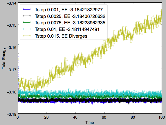
Fig 8 shows the equilibrium energy for the system as calculated with each timestep. It can be seen that a timestep of 0.015 is far from suitable as, with this timestep, the system does not equilibrate. All the other timesteps results in systems that reach equilibrium at very similar total energies (range <1%). However, there appears to be a pairing of equilibration energies. The timesteps of 0.001 and 0.0025 equilibrate about -3.184 whereas the two other equilibrating timesteps result in systems with total energies of -3.182 and -3.181 for the timesteps 0.0075 and 0.01 respectively. The smaller the timestep, the greater the number of steps run for a given total time, this increases the computational cost. It is decided that a suitable compromise would be to select a timestep of 0.0025 as it produces extremely similar results to those of smaller timesteps but has a lower computational cost than the 0.001 timestep. Tick, correct

Running Simulations Under Specific Conditions

Solving for $\gamma$

Given that….

$\frac{1}{2}\sum _i{m}_i{v}_i^2=\frac{3}{2}N{k}_{B}T$

and…

$\frac{1}{2}\sum _i{m}_i{\left(\gamma v_i\right)}^2=\frac{3}{2}NkB\mathfrak{𝔗}$

Summing the two equations gives…

$\frac{1}{2}\sum _i{m}_i{v}_i^2+\frac{1}{2}\sum _i{m}_i{\left(\gamma v_i\right)}^2=\frac{3}{2}N{k}_{B}T+\frac{3}{2}NkB\mathfrak{𝔗}$

Take out constant \gamma^2 and common factors…

$\frac{1}{2}\sum _i{m}_i{v}_i^2(1+{\gamma }^2)=\frac{3}{2}N{k}_B(T+\mathfrak{𝔗})$

Sub in $\frac{1}{2}\sum _i{m}_i{v}_i^2=\frac{3}{2}N{k}_{B}T$ …

$\frac{3}{2}N{k}_{B}T(1+{\gamma }^2)=\frac{3}{2}N{k}_B(T+\mathfrak{𝔗})$

Cancel and rearrange…

${\gamma }^2=\frac{\mathfrak{𝔗}}{T}$

Finally…

$\gamma =\sqrt{\frac{\mathfrak{𝔗}}{T}}$ Tick

LAMMPS Commands II

Importance of the three numbers 100, 1000 and 100000.

Nevery -> 100 – In this case the computer will sample input values every 100 timesteps

Nrepear -> 1000 – Use input values 1000 times to calculate averages

Nfreq -> 100000 – Instructs the computer to calculate averages every 100000 timesteps

The number of measurements that contribute to the average is…

$N_{Measurements}=\frac{N_{Timesteps}}{Nevery}$

So…

$N_{Measurements}=\frac{100000}{100}=1000$

The amount of time simulated will be…

$Time=N_{Timesteps}*Timestep$

So…

$Time=100000*0.0025=250$ Tick

Plotting the Equations of State

Fig 9. shows Number Density Vs Temperature for the simulation and as predicted by the ideal gas law for the pressure 2.5 and 3.0

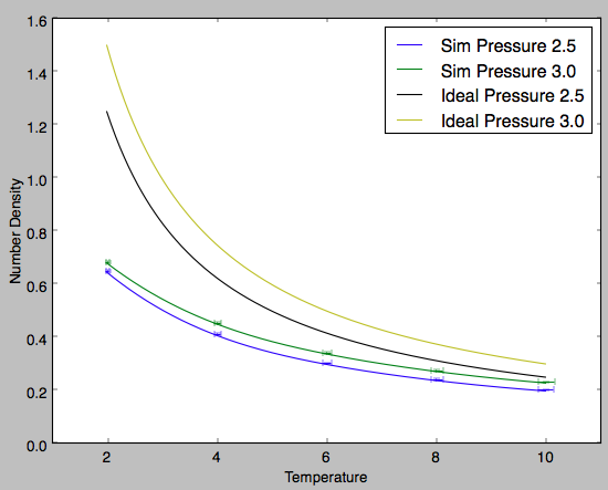
The two selected reduced pressure were 2.5 and 3.0. They were selected as they were within the range of the fluctuations of the pressure vs time graph once the system reached equilibrium. From the graph two observations are clear: at higher temperatures the simulated number density is in stronger agreement with the ideal gas law and at lower pressures the difference between the simulated number density and that predicted by the ideal gas law is less.

The ideal gas law is based on several assumptions. 1) The gas consists of small hard spheres and therefore all collisions are perfectly elastic 2) The total volume of all the molecules is much smaller than the volume occupied by the gas 3) There are no interactions between particles outside of perfectly elastic collisions

This assumptions are the source of the differences between the simulated and theoretical plots. At lower temperatures the gas occupies a smaller volume and begins to degrade assumption 2. However, this effect is small considering the temperatures at which the simulations are being run. However, given the gas occupies a smaller volume the particles are in much closer to proximity to eachother. Assumption 3 dictates that there are no electrostatic intermolecular interactions but this is simply not the case and at lower temperatures the error in this assumption is magnified. Hence, the larger difference between the simulated values and the theoretical values at lower temperature. The same reasoning can be applied to the divergent character of the two plots with increasing pressure. A larger pressure results in a smaller volume occupied by the gas and this magnifies the errors observed in assumptions 2 and 3. Furthermore, it can be said that at higher temperatures and lower pressures the simulated gas exhibits more perfect gas character. This is expected and is true of all gases and so it adds evidence that this simulation was successful and at least qualitatively accurate. Tick, good

Calculating Heat Capacities

Below is an example input script that was used for the subsequent simulations. In this script the density was set to 0.8 and temperature to 2.8.

### DEFINE SIMULATION BOX GEOMETRY ###
variable dens equal 0.8
lattice sc ${dens}
region box block 0 15 0 15 0 15
create_box 1 box
create_atoms 1 box

### DEFINE PHYSICAL PROPERTIES OF ATOMS ###
mass 1 1.0
pair_style lj/cut/opt 3.0
pair_coeff 1 1 1.0 1.0
neighbor 2.0 bin

### SPECIFY THE REQUIRED THERMODYNAMIC STATE ###
variable T equal 2.8
variable timestep equal 0.0025

### ASSIGN ATOMIC VELOCITIES ###
velocity all create ${T} 12345 dist gaussian rot yes mom yes

### SPECIFY ENSEMBLE ###
timestep ${timestep}
fix nve all nve

### THERMODYNAMIC OUTPUT CONTROL ###
thermo_style custom time etotal temp press
thermo 10

### RECORD TRAJECTORY ###
dump traj all custom 1000 output-1 id x y z

### SPECIFY TIMESTEP ###

### RUN SIMULATION TO MELT CRYSTAL ###
run 10000
unfix nve
reset_timestep 0

### BRING SYSTEM TO REQUIRED STATE ###
variable tdamp equal ${timestep}*100
variable pdamp equal ${timestep}*1000
fix nvt all nvt temp ${T} ${T} ${tdamp}
run 10000
reset_timestep 0

unfix nvt
fix nve all nve

### MEASURE SYSTEM STATE, atoms will output atom number###
thermo_style custom step etotal temp press density atoms
variable atoms equal atoms
variable E equal etotal
variable E2 equal etotal*etotal
variable dens equal density
variable dens2 equal density*density
variable temp equal temp
variable temp2 equal temp*temp
fix aves all ave/time 100 1000 100000 v_E v_dens v_temp v_E2 v_dens2 v_temp2
run 100000

variable aveE equal f_aves[1]
variable avedens equal f_aves[2]
variable avetemp equal f_aves[3]
variable aveE2 equal f_aves[4]
variable errdens equal sqrt(f_aves[5]-f_aves[2]*f_aves[2])
variable errtemp equal sqrt(f_aves[6]-f_aves[3]*f_aves[3])
variable CV equal (${atoms}*${atoms})*((${aveE2}-(${aveE}*${aveE}))/(${avetemp}*${avetemp}))
variable vol equal vol
variable y equal ${CV}/${vol}

print "Averages"
print "--------"
print "Density: ${avedens}"
print "Stderr: ${errdens}"
print "Temperature: ${avetemp}"
print "Stderr: ${errtemp}"
print "Heat Capacity: ${CV}"
print "CV/V: ${y}"

Fig 10. shows Cv/V Vs Temperature for densities of 0.2 and 0.8

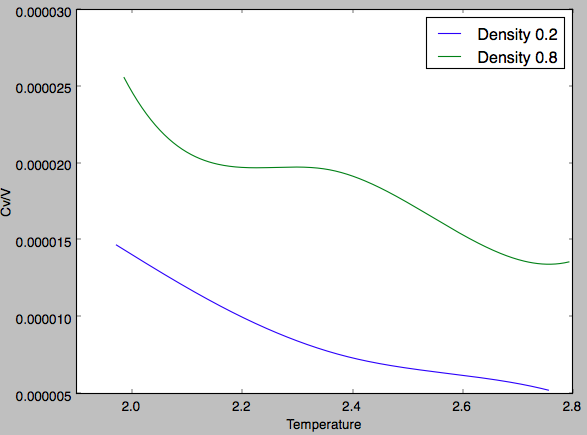
Once again two trends are clear, the first that with increasing density the heat capacity per unit volume increases and the second being that with increasing temperature there is a general decrease in the heat capacity per unit volume. The first observation can be explained by the fact that there are more atoms per unit volume. The volumetric heat capacity being the thermal energy required to a unit volume of the system by a degree Kelvin. For a more dense system, there are more atoms over which this heat energy is 'shared' and so more thermal energy is required to raise the temperature of the substance. The second observation is explained when the structure of the energy levels is considered. There is a maximum and minimum possible energy level independent of system size and the energy levels inbetween are not spread out evenly. There is a higher density of states towards the maximum energy level, this results in smaller energy gaps between quantised levels as higher energy levels are occupied. This occurs at higher temperatures as the system has more energy and so with increased temperature the energy required to excite to the next energy level decreases. Therefore, the volumetric heat capacity decreases with increasing temperature. However, there will come a point at which all the energy levels are equally occupied and it is not possible to have more populated higher energy levels and so the heat capacity at very high temperatures will eventually become infinitely large. For the plot of number density 0.8, midway through the line the plot deviates from the general decreasing trend. There are a number of reasons why the volumetric heat capacity may change, for example phase change or conformational change. However, in this case as the increase in heat capacity is small it is likely that at this temperature for this density a new rotational or vibrational energy level of the liquid is accessed. Therefore, the heat energy put into the system doesn't manifest itself as translational kinetic energy and thus, does not contribute to the temperature. Hence, the increase in volumetric heat capacity. Tick, nice explanation. I especially liked your reasoning for the anomaly

Structural Properties and the Radial Distribution Function

Fig 11. shows the radial distribution function for the three phases solid, liquid and vapour

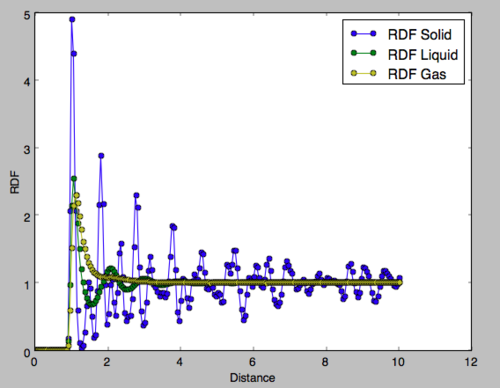
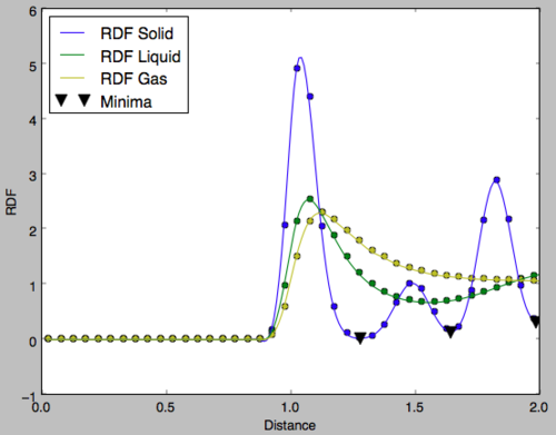
It can be seen that for inter-particular distances less than 1, the radial distribution function is zero for all phases. This is because of the repulsion between molecules as the get very close together and so no phase will exhibit particles at this proximity. The radial distribution functions of the three phases after this point are very different and give a picture of the structure of each phase.

Gas RDF

There is an initial peak where the nearest particle is most likely to be found and from there the RDF tends to one. This value of one indicates the normalised density of the phase and not the number density. This displays the lack of long and short-range order in a gas. Multiple peaks would indicate the presence of particles at specific distances but in this case it is clear that other molecules can appear at any distance from the observed particle simply with decreasing probability. This highlights the disorder in the gaseous phase. Tick

Liquid RDF

In the liquid phase, three peaks are observed each of decreasing integration and increasing width. These correspond to the spheres of coordination around the observed particle. The first coordination sphere has stronger intermolecular interactions with the central molecular and is therefore more ordered leading to a sharper peak in the RDF. With increasing distance the intermolecular interactions become weaker and so the number of molecules in each coordination sphere decreases. Furthermore, the order of the sphere becomes less apparent and the sphere has a larger radius, hence the increased width of the peak. After the third peak the RDF tends to the density and the lack of long-range order is observed.Tick, what about the relative smoothness of the rdf relative to solid?

Solid RDF

Fig 12. shows the FCC structure of the solid phase with arrows indicating the 3 first peaks in the RDF

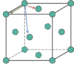
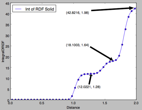
In the solid phase, the peaks do not correspond to spheres of coordination but to particle positions on the FCC framework of the solid. It can be seen that peaks are observed even at a distance of 10 units indicating the long-range order of the solid. Fig 13 shows the region of the first 3 peaks for the solid RDF, the x-values of the minima are obtained as the integral at these points should correspond to the number of filled lattice sites at that distance in 3D. For an FCC lattice, imagining Fig 12 in three dimensions, 12 sites would be expected at an absolute distance of the red vector, 6 for the green and 24 for the blue. In Fig 14, the y-value is the integral of the RDF indicating the total number of molecules from a distance of 0 up to the x-value, therefore, subtracting the y-value of each peak from the last would give the number of atoms for each peak. It is clear that the integral of the RDF is in extremely strong agreement with what was expected from an FCC lattice. The red arrow corresponds to the set of lattice vectors [0.5, 0.5, 0], the green [1, 0, 0] and the blue [1, 0.5, 0.5]. Good

Fig 13. is a zoomed image of Fig 11 with the x-values of the minima obtained for the solid RDF

Fig 14. shows the running integral of the radial distribution function for the solid phase

Dynamical Properties and the Diffusion Coefficient

In the following exercise, output files for 1,000,000 particles was given for comparison. The linear region of each plot is the region in which diffusion is the only factor affecting the MSD. The value of the gradient will indicate the level of diffusion. In Fig 15, a sharp increase in the MSD is observed and then the gradient tends to 0. This shows that for the solid there is some initial small rearrangement from the FCC lattice defined and then the particles are confined and there is no diffusion.

Fig 15. shows the MSD Vs Number of Timesteps for the solid phase

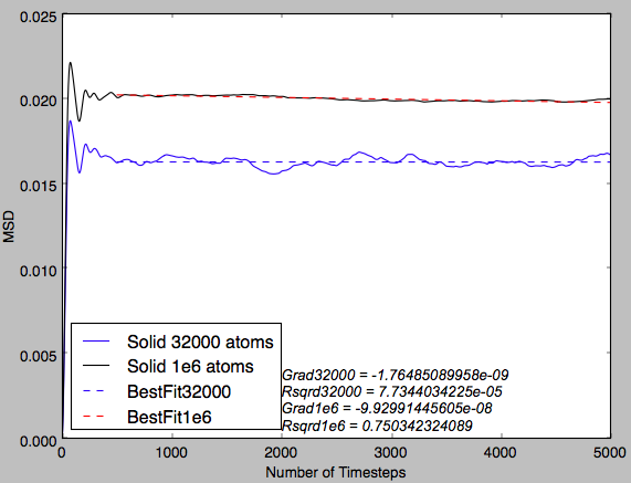
Fig 16 shows a near-perfect straight line plot for both system sizes. This indicates that diffusion is the only phenomenon observed in this plot.

Fig 16. shows the MSD Vs Number of Timesteps for the liquid phase

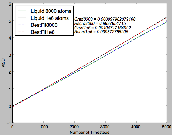
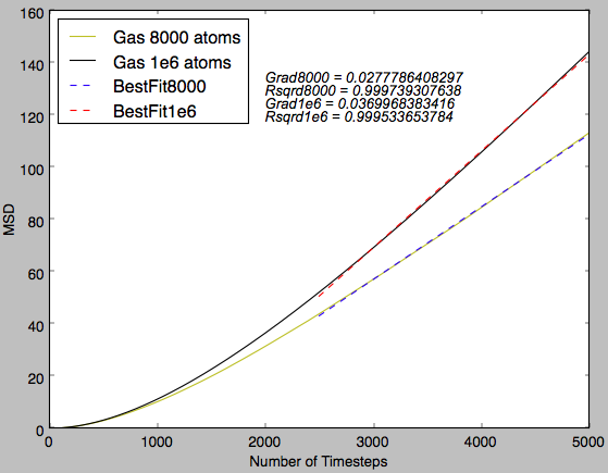
Fig 17 indicates that there is an initial curve in the plot before the linear region is observed. This indicates that there is a force observed in the system and diffusion is not the only factor affecting the MSD at the start of the simulation. This is probably due to a higher number of collisions between particles due to the organised starting positions and this exhibits an increased pressure that results in this initial curving of the plot. Tick

Fig 17. shows the MSD Vs Number of Timesteps for the gas phase

MSD Gradient Analysis

In the table below the gradients of the plot were converted into the diffusion coefficient by diving by the timestep, ie converting number of timesteps into time and diving by 6 (multiplying the gradient by 0.5 for each dimension). It can be seen for the solid that the diffusion coefficient is effectively zero, indicating that the atoms are fixed in position and that there is no diffusion. Then for the next two phases increasing magnitudes of diffusion coefficient are observed. This qualitatively shows the increasing ease with which a particle can diffuse through each phase. Furthermore, it can be seen that for a greater system size there is significantly smoother plots. This shows that the smaller system size, despite requiring a shorter computational run-time, is significantly less accurate and the result is plots that are noisy in appearance and diffusion coefficients that are only qualitatively accurate.Tick

Phase	Diffusion Coeff 8000/32000 atoms	Diffusion Coeff 1000000 atoms
Solid	-1.10*10-7	-8.27*10-6
Liquid	0.0832	0.0873
Gas	2.32	3.08

Normalised VACF for 1-D Harmonic Oscillator

The equations for the VACF...

$C\left(\tau \right)=\frac{\underset{-\mathrm{\infty }}{\overset{\mathrm{\infty }}{\int }}v\left(t\right)v(t+\tau )\mathrm{d}t}{\underset{-\mathrm{\infty }}{\overset{\mathrm{\infty }}{\int }}{v}^2\left(t\right)\mathrm{d}t}$

The displacement as a function of time for the harmonic oscillator...

$x(t)=Acos(\omega t)$

Therefore velocity is the integral of the displacement...

$v(t)=-A\omega sin(\omega t)$

Subbing in to the equations for VACF and using trig identities...

$C\left(\tau \right)=\frac{\underset{-\mathrm{\infty }}{\overset{\mathrm{\infty }}{\int }}sin(\omega t)(sin(\omega t)cos(\omega \tau )+sin(\omega \tau )cos(\omega t)\mathrm{d}t}{0.5\underset{-\mathrm{\infty }}{\overset{\mathrm{\infty }}{\int }}(1-cos(2t))\mathrm{d}t}$

Using the following results...

1) $\underset{-\mathrm{\infty }}{\overset{\mathrm{\infty }}{\int }}si{n}^2(\omega t)=0.5(t-\frac{sin(2\omega t)}{2\omega }{)}_{-\mathrm{\infty }}^{\mathrm{\infty }}$

2) $\underset{-\mathrm{\infty }}{\overset{\mathrm{\infty }}{\int }}sin(\omega t)cos(\omega t)=\frac{si{n}^2(\omega t)}{2\omega }{)}_{-\mathrm{\infty }}^{\mathrm{\infty }}$

Using these results...

$C\left(\tau \right)=\frac{{\{\frac{cos(\omega \tau )}{2}(t-\frac{1}{2\omega }sin(2\omega t))+\frac{sin(\omega \tau )}{2\omega }si{n}^2(\omega t)\}}_{-\mathrm{\infty }}^{\mathrm{\infty }}}{{\left\{\frac{1}{2}(t-\frac{1}{2\omega }sin\left(2\omega t\right))\right\}}_{-\mathrm{\infty }}^{\mathrm{\infty }}}$

Because sin(t) is an odd function and sin²(t) is symmetric about the y-axis the functions are equal to 0 so...

$C\left(\tau \right)=\frac{0.5cos(\omega \tau )[t{]}_{-\mathrm{\infty }}^{\mathrm{\infty }}}{0.5[t{]}_{-\mathrm{\infty }}^{\mathrm{\infty }}}$

Again equal divergences so $[t{]}_{-\mathrm{\infty }}^{\mathrm{\infty }}$ can cancel...

$C\left(\tau \right)=cos(\omega \tau )$ Tick

Plots

Below the theoretical C(t) for the 1-D harmonic oscillator was plotted with the simulated VACF-Number of timestep plots for the solid and liquid phases. The VACF plot shows the molecular dynamics that occur in the structure. It can be seen that within the solid due to the oscillating nature of the VACF there is some level of vibrational energy in the lattice. In the liquid VACF plot, the first minimum indicates some repulsion between two particles and the rest of the plot shows their separation as a result of their new velocities and diffusion. Not quite, think more about what the correlation function represents - the velocity correlation function provides vital information as to how the velocity at a time t+dt will essentially 'depend' on the velocity at time t. If a particle collides, it changes velocity and the VACF will also change. The first minimum can be described as the point at which all the particles have first collided...

Fig 18. shows the VACF Vs Number of Timesteps for the solid and liquid phases and the analytical theoretical solution

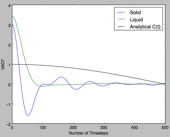
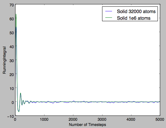
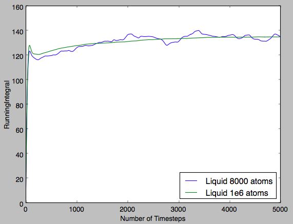
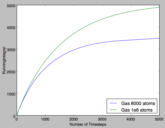
Using the VACF plot the diffusion coefficient can be calculated by integrating the plot. Figures 19, 20 and 21 show this for the three phases.

$D=\frac{1}{3}\underset{0}{\overset{\mathrm{\infty }}{\int }}\mathrm{d}\tau ⟨\mathbf{v}\left(0\right)\cdot \mathbf{v}\left(\tau \right)⟩$

The table below shows the estimated value of the diffusion coefficient using the Simpson's rule to integrate the plots. Qualitatively, it shows the exact same trend as the MSD plots did. However, the values for the diffusion coefficient are vastly different. The largest source of error is quite clearly the system size, as it has been observed throughout all of the MSD and VACF plots the smaller system size results in vastly different values for the diffusion coefficient, particularly in the gas phase and the plots are rather noisy and one can immediately discard any sort of quantitative analysis as a result. However, it would appear that the simulation is most valid for liquids and the discrepancy between the results is quite small. Furthermore, Molecular Dynamics is a classical approach to model structures but in reality there are quantum mechanical contributions, like the zero-point energy. This is another source of error that is introduced in this simulation and an error that increases in size with decreasing temperature. Finally, it is not believed that a large amount of error results from the approximate integration as an extremely large number of 'slices' were taken for the Simpson's rule and so it is believed that the value obtained is very close to the actual integral.Tick, nice

Phase	Diffusion Coeff 8000/32000 atoms	Diffusion Coeff 1000000 atoms
Solid	0.0941	0.0228
Liquid	45.0	45.0
Gas	1170	1634

Fig 19. shows the running integral of the solid phase VACF

Fig 20. shows the running integral of the liquid phase VACF

Fig 21. shows the running integral of the gas phase VACF