Rep:FabianThomasThirdYearMgOSimulation

Abstract

Lattice Dynamics (LD) simulations using the quasi-harmonic oscillator approximation (QHA), and Molecular Dynamics (MD) simulations were carried for MgO over a range of temperatures using GULP. The phonon dispersion, density of states and thermal expansion coefficients were investigated in order to understand how a change in temperature affected the volume of MgO. It was found that a 16x16x16 grid was the optimal grid size for carrying out LD simulations. The lattice parameter and volume increased polynomially with temperature for LD simulations, while was more linear with MD simulations. Thermal expansion coefficients were calculated from 50-2900 K for LD and 50-3700 K for MD. MD was found to be better at simulating temperatures less than 700 K, while LD was more accurate above 700 K for calculating the thermal expansion coefficient of MgO. With values for the thermal expansion coefficient of 20.53 x 10^-6 K^-1 and 25.82 x 10^-6 K^-1 at 300 K, and 35.23 x 10^-6 K^-1 and 30.33 x 10^-6 K^-1 at 1200 K for LD and MD respectively.

Introduction

One of the earliest uses of thermal expansion in daily life was the mercury thermometer. A change in temperature would lead to the mercury either taking up more or less space depending on if it became hotter or colder, thus allowing the temperature to be measured. Thermal expansion is seen in a variety of sectors in daily life, one major sector being the transportation sector. At high temperatures, train tracks which have not been built with thermal expansion in mind buckle due to the expansion of the metal. This can lead to delays, closing of railways, or in the worst case the derailment of a train due to the sharp angles of the buckled train tracks. Many motorways around the world now have expansion joints made of metal teeth that fit together, which when the temperatures rise the metal teeth in the joints expand to fill the empty space instead of cracking the road. Thus the expansion of materials under a change in temperature is an important aspect of research for many sectors in the world.

Modelling thermal expansion using Lattice Dynamics and Molecular Dynamics and understanding the phonon modes of a material allows for the comparison between two types of simulation and the study of thermal expansion of materials. This means that possibly expensive experiments to determine this property experimentally will not be needed to test the viability of a material for use. Some of the most commonly used materials such as steel or concrete vary in composition depending on what application the material is being used for, and so simulations similar to the ones carried out in this experiment can be used to determine the qualities of the material and what type of composition it needs to have, before production. Even though these simulations are powerful, there are questions still unanswered, how complex a system can these methods accurately simulate and are there any types of material that these simulations cannot compute?

Theory

The quasi-harmonic approximation for phonons builds upon the harmonic approximation for phonon dynamics, and therefore to explain the quasi-harmonic approximation we must first discuss the harmonic approximation.

For a regular, linear chain which is composed of $N$ number of particles, the forces between a pair of atoms can be assumed to be a potential energy function $V$ which depends on the distance of the separation between the atoms. The main contributing forces to the potential are described by an electric force, such as electrostatic attractions, covalent bonds or Van der Waals forces. Therefore the potential energy of the entire lattice made up of $N$ atoms is the sum of the potential energies between each pair of atoms with a separation r from each other shown below in Equation 1.

$E=NV(r)$ $(1)$

Now, allowing each atom to deviate slightly from its equilibrium position by a displacement $u$, if the deviations are small in comparison to the distance between each atom $r$, the energy of this chain is able to be calculated via a Taylor expansion summing over all of the atoms in the chain.

$E=NV+\sum _{s\ge 1}\frac{1}{s!}\frac{{\partial }^{s}V}{\partial u^s}\sum _n(u_n-u_{n+1}{)}^s$ $(2)$

Where $u_n$ is the displacement of the $n$th atom from its equilibrium position.

Two approximations are used in order to reach this equation, which together forms the harmonic approximation and it's respective equation. The first approximation states that the sum of the pair potential energies is completed over only neighbouring atoms, as although there are electric forces between all atoms, these forces on atoms far away from one another are greatly diminished by screening by the atoms in between. The second approximation is that the potential energies are treated as harmonic potential energies. In this equation, the first derivative is zero, whereas higher order terms are not, and so the first term can be dropped, and the second term is used where $s=2$, with higher order terms being neglected. These higher order terms are ignored as harmonic equations of motion have exact solutions, while anharmonic equations do not have exact solutions to them and require more approximations. Thus the energy of the lattice is the same as the energy of the set of harmonic oscillators. The error in this equation remains small for small values of $u$ as the value of higher order terms will remain low.

The quasi-harmonic approximation expands upon the harmonic approximation by taking into account some of the true anharmonicity of the interactions between atoms. The quasi-harmonic approximation relates the Hemholtz free energy of a perfect lattice to both its temperature and its volume, in contrast to the harmonic oscillator approximation which only depends on temperature as shown in Equation 3ː

$F=E_0+\frac{1}{2}\sum _{k,j}^{}\hslash {\omega }_k+k_{B}T\sum _{k,j}^{}ln(1-e^{\frac{-\hslash {\omega }_k}{k_{B}T}})$ $(3)$

Where $F$ is the Hemholtz free energy and $E_0$ is the lattice energy

As this definition of the free energy also takes into account the volume of the lattice, this allows thermal expansion to be calculated as it allows the harmonic approximation to hold for all temperatures.

Molecular Dynamics simulates a lattice of atoms using Newton's equations of motion and so simulates the cell over a certain period of time, taking a time-average of the cell to obtain physical quantities. In the simulations run in this experiment, an isothermal-isobaric (NPT) ensemble was used to calculate the thermal expansion coefficients and volume of the MgO cell at specific temperatures. As MD is based on Newton's laws of motion it does not take into account quantum effects such as the zero-point energy of a material in comparison to QHA which does.

Results and Discussion

Phonon modes and Free Energy of MgO

Figure 1: A phonon dispersion plot for MgO

Figure 2: A plot of the density of states for MgO using a 1x1x1 grid size

Figure 3: The optimised plot of the density of states for MgO using a 16x16x16 grid size

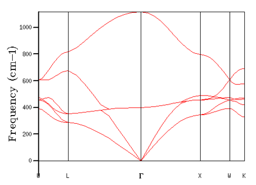
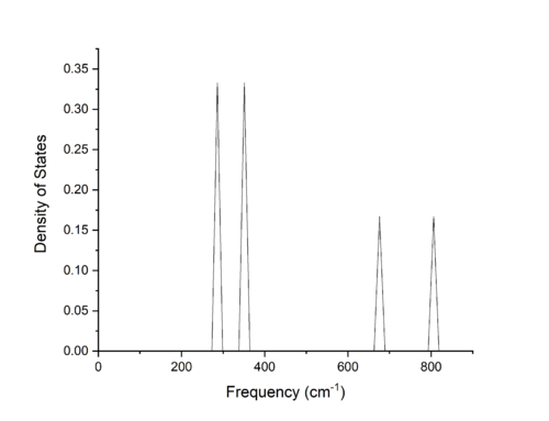
From Figures 1 and 2, we can see the computed phonon dispersion curve and density of states for a 1x1x1 grid size containing one k-point. Correlating the density of states with the dispersion curve via their shared axis of frequency of vibration yields the k-point L on the dispersion curve as the singular k-point used for the calculation. The density of states shows bands at 286 and 351 cm^-1 and 676 and 806 cm^-1, with the intensities of the first two bands double that of the final two bands. These bands correspond to three acoustic and three optical branches, with the first two bands of 0.333 intensity corresponding to a k-point where two branches are overlapping and are therefore degenerate states.

Varying the grid size used for the calculation greatly affected the accuracy and precision of the results of calculations through increasing the number of k-points sampled in Equation 4ː

${\omega }^2(k)=C(\frac{1}{M_{Mg}}+\frac{1}{M_O})\pm \sqrt{(\frac{1}{M_{Mg}}+\frac{1}{M_O}{)}^2-\frac{4si{n}^2(ka)}{M_{Mg}}}$ $(4)$

Where $C$ is the spring force constant, $M_{Mg}$ is the molar mass of magnesium and $M_O$ is the molar mass of oxygen

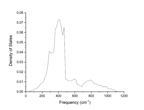
As the grid size increases, and thus the more k-points sampled, more and more features become visible, with the increase in number of points sampled along the dispersion curve leading to the increase in number of bands seen in the density of states. Optimising the grid size led to a grid size of 16x16x16 being chosen. As expected, the density of states plot produced from this grid size was smooth, as can be seen in Figure 3. This curve was proved to be a good optimisation through looking at the Hemholtz free energy for each of the simulated grid sizes. As the accuracy of the Helmholtz free energy result directly depends on the number of k-space points sampled in the calculations as can be seen in Equation 2. Similarly to Equation 4, the larger the grid size, and therefore the more k-points sampled, the more accurate the result. Comparing the free energy of the 16x16x16 grid to the 32x32x32 grid; which for higher order grids remained constant and so had converged, the 16x16x16 was accurate to within 0.001 meV or 2.4434 × 10^-6 %.

In comparison to smaller grid sizes, the 16x16x16 grid size curve appears more smooth, and more akin to a single band as seen for macrostructures. Larger grid sizes, while greatly increasing the computation time of the calculation did not largely increase the accuracy of the calculations as stated above, and therefore the 16x16x16 grid size was the optimal choice for these simulations.

Table 1. Calculated Total Difference in Hemholtz Free Energy

Grid Size	Total Difference in Free Energy
1	3.818
2	0.126
3	-0.051
4	-0.033
8	-0.005
16	-0.001
24	-0.000
32	0.000
64	0.000

Table 1 shows the difference between the calculated free energy for grid size and the final converged free energy. Looking at this, we can see that for grid sizes larger than 24x24x24, there is no change in the free energy of the system and so the free energy has converged to a minima, although it may not be the global minimum. The accuracy of simulations also increase rapidly with grid size, for example for accurate simulated energies to 1, 0.5 and 0.1 meV per cell, grid sizes of 2x2x2, 4x4x4 and 8x8x8 respectively can be used. This rapid increase in the accuracy of the calculation can be attributed to the large increase in k-points sampled over within the summations in Equation 2 with increasing grid size.

However, the optimal grid size dependent on the material used due to the relationship between the lattice parameter, and the size of the first brillouin zone in k-space. For a similar oxide such as CaO, in comparsion to the lattice parameter of MgO of 4.212 Å , the parameter of CaO is 4.864 Å , slightly larger than that of MgO. This leads to a slightly smaller grid size being optimal, as the larger lattice parameter leads to a smaller brillouin zone in reciprocal space as if the lattice parameter $a$ is larger, then the size of the first brillouin zone $a^{*}=\frac{2\pi }{a}$will be smaller. This in turn allows less points to be sampled inside the region to give the same spacing of points, and therefore accuracy for the density of states as for MgO. Similarly, the zeolite faujsite has an extremely large lattice parameter of 25.132 Å , in comparison to MgO. This; as with the case of CaO but more exaggerated, leads to a much smaller brillouin zone in reciprocal space, and so allows for a much smaller grid size to give the same accuracy as the MgO calculation due to the extremely small value of $a^{*}$ obtained for faujsite. Conversely, lithium has a smaller lattice spacing of 3.51 Å . Therefore the value of $a^{*}$ for lithium will be larger than for MgO, and so require a larger grid size to obtain the same spacing between sampled k-space points and therefore the accuracy of the calculated density of states.

Thermal Expansion of MgO

Figure 4: A plot of lattice parameter against temperature for MgO

Figure 5: A plot of lattice volume against temperature for MgO, with the magenta line on the graph corresponding to the polynomial fit for the graph, and the red point the points which were not fitted over

Figure 6: A plot of free energy against temperature for MgO

The physical origin of thermal expansion for a solid lattice arises from the increase of kinetic energy of a material with an increase in temperature. All atoms within a lattice vibrate and move about their positions within the lattice and with an increase in temperature, each atom in the lattice gains kinetic energy, increasing the strength of its vibrations and the speed at which the atoms move. Due to this, the atoms on average take up more space at higher temperatures than lower temperatures and so averaged out over many atoms in a lattice, this increases the volume of the lattice.

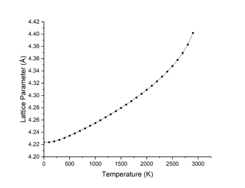
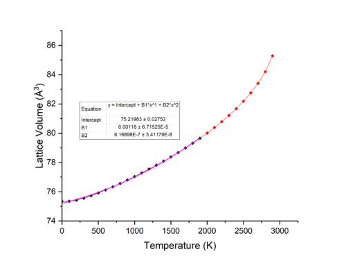
Figures 4 & 5 show the effect of change of temperature on the lattice parameter and volume of MgO in the range of 50-2900 K. As we can seen from the figures, from 50-400 K, a change in temperature does not largely increase the volume, while above 400 K the trend seems to be linear with respect to volume increase through an increase in temperature. This is however not the case at higher temperatures above 2200 K where the trend is more polynomial in nature.

Figure 6 shows the effect of change in temperature on the Hemholtz free energy of MgO. From 50-400 K, the dominating term for the free energy is the zero point energy, and thus a change in temperature does not greatly change the free energy of the lattice and so volume changes at low temperatures are minimal. At temperatures above 2200 K not only is the entropic term completely dominating all other terms for the free energy, but also higher order anharmonic terms for the free energy that were excluded in the harmonic approximation part of the equation begin to play a large role in the free energy. This leads to the gradient no longer being linear.

The thermal expansion coefficients for MgO can be calculated through using the gradient $(\frac{\partial V}{\partial T}{)}_p$ at a specific value of $T$ in the equationː

$\alpha =\frac{1}{V_i}(\frac{\partial V}{\partial T}{)}_p$ $(5)$

Where $\alpha$ is the coefficient of thermal expansion, $V_i$ is the volume of the lattice at 0 K and $(\frac{\partial V}{\partial T}{)}_p=6.16898\times 10^{-7}T+0.00118$

Table 2 displays thermal expansion coefficients for the polynomial fit of MgO, alongside the temperature range that the fit was made over.

Table 2. Calculated Linear fit Thermal Expansion Coefficients for MgO

Temperature (K)	Thermal Expansion Coefficient (x 10-6 K-1)	Temperature (K)	Thermal Expansion Coefficient (x 10-6 K-1)
50	16.44	1500	40.13
100	17.26	1600	41.76
200	18.89	1700	43.40
300	20.53	1800	45.03
400	22.16	1900	46.67
500	23.79	2000	48.30
600	25.43	2100	49.93
700	27.06	2200	51.57
800	28.69	2300	53.20
900	30.33	2400	54.83
1000	31.96	2500	56.47
1100	33.60	2600	58.10
1200	35.23	2700	59.74
1300	36.86	2800	61.369
1400	38.50	2900	63.00

As we can see from the table of results, the coefficient of thermal expansion is not independent of temperature, but changes with it. In comparison to literature values, at 300 K the data obtained through this experiment largely agrees with the literature data of a value for the thermal expansion coefficient of 35.73 x 10^-6 K^-1

Deviations from the literature values can be attributed to shortcomings of the quasi-harmonic oscillator approximation. The main approximation being that the oscillations of the atoms about their equilibrium positions are small, which for higher energy phonon modes is not representative of those modes. It is seen that the difference in our calculated values to that of literature values decreases as the temperature increases such that for a literature value of 42.51 x 10^-6 K^-1 at 1200 K, our calculated value is 35.23 x 10^-6 K^-1.

At temperatures above the melting point of MgO - 3125 K - the phonon modes of MgO are not accurate represented. This is due to the fact that above this temperature MgO melts from a solid to a liquid, and thus the approximation that the solid is a perfect lattice breaks down. This means that for temperatures near to or above 3125 K the data is not representative of the true phonon modes as a solid is being simulated whereas in reality the material is already is a liquid and so solid phonon modes cannot describe the liquid modes.

Although the quasi-harmonic approximation breaks down at higher temperatures, unlike other approximations such as the harmonic approximation, it can be used to model thermal expansion. Consider a diatomic harmonic oscillator, with an increase in temperature the strength of oscillation will increase, but in equal proportions relating to lengthening and contracting of the bond due to the nature of a harmonic potential. This leads to an increase in temperature not changing the equilibrium bond length and thus thermal expansion cannot be modelled. The quasi-harmonic approximation takes into account some of the anharmonic nature of the true bond and so allows thermal expansion to be modelled. This can be visualised through viewing a morse potential. A contraction of bond length in a morse potential require a much larger amount of energy than an increase in bond length, therefore at higher temperatures and so higher energies, while the bond length maximum will largely increase, the minimum bond length will change only slightly, thus on average the bond length will have lengthened. This leads to an increase in equilibrium bond length, and so applying this so a lattice leads to an increase in volume of the lattice.

Molecular Dynamic Simulations

Figure 7: A plot of cell volume against temperature for the molecular dynamics calculations

Figure 8: A plot of cell volume against temperature comparing the values calculated via Molecular Dynamics and Lattice Dynamics

Figure 9: A plot of the thermal expansion coefficient for both Molecular Dynamics and Lattice Dynamics simulations

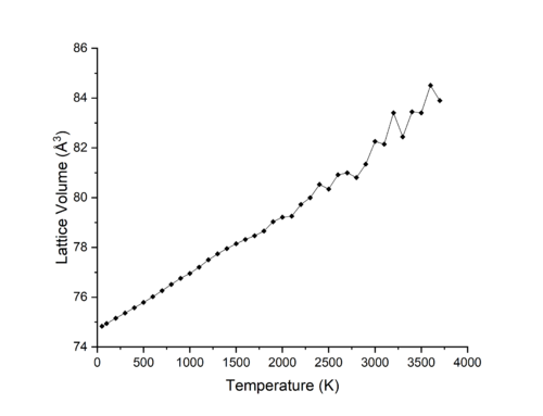
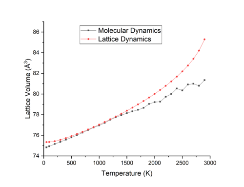
Molecular dynamics simulations were run using from 50-3700 K as shown in Figure 7. Figures 8&9 compare the results of Molecular dynamics and Lattice Dynamics (quasi-harmonic approximation) simulations. In Figure 8 it is seen that the difference in volume the MD and LD plots for the range 400-1400 K is quite small, while at temperatures lower than 400 K and higher than 1400 K the simulations begin to deviate from each other. Figure 9 compares the calculated coefficient for thermal expansion for MD and LD, taking a value at 300 K of 25.82 x 10^-6 K^-1 and 30.33 at 1200 K, in comparison to the literature values of 35.73 x 10^-6 K^-1 at 300 K and 42.51 x 10^-6 K^-1 at 1200 K, it can be seen that at lower temperatures, the MD approach is more accurate, while at higher temperature LD is more accurate. As MD calculations average the volume of the cell over set intervals - the timestep - for a set period of time, the erractic nature of the MD curve at high temperatures in Figure 8 is due to the large velocities of the ions in the lattice which leads to the timestep being too large to take an accurate snapshot of the system and its variations. Thus a timestep smaller than the 500 fs interval used would reduce the noise in the simulation and provide a more accurate description of the volume at higher temperatures.

LD and MD simulations differ due to the differences between how they calculate their results and the approximations they take into account. MD differs from LD at lower temperatures due to the lack of higher order quantum corrections which LD takes into account, while at higher temperatures MD should be more accurate due to the use of Newton's classical equations which dominate all quantum effects, while LD should suffer from a lack of higher order anharmonic terms in its approximation. . In spite of this, LD produces more accurate results at higher temperatures, while MD is more accurate at lower temperatures.

As stated above, at temperatures near to or larger than the melting point of MgO, a LD simulation fails to produce accurate results for the volume of the cell due to the fact that a solid is still being simulated rather than a liquid. MD simulations however work through Newton's laws of motion and so can model phase transitions of materials. This can be seen in Figure 7, where after the melting of MgO at 3125 K the change in volume per 100 K is larger than for temperatures below this point, due to the forces between liquid molecules being weaker than that of solids, and so thermal expansion of liquids is larger than solid for the same change in temperature.

Conclusion

Through modelling of MgO through LD and MD simulations, the phonon distribution and density of states was calculated and a 16x16x16 grid size was found optimal for LD simulations. For LD simulations, lattice volume was found to at first increase linearly, but after 1700 K increase in a more harmonic or polynomial form with temperature. Similarly for the Hemholtz free energy, the increase in free energy was found to be more linear at first, and then become more polynomial in nature above 1700 K. LD thermal expansion coefficents were found to follow a polynomial trend, following a linear trend to 2200 K but diverging after this point to a more polynomial nature. MD simulations for the change in volume of MgO against temperature were linear throughout the temperature range sampled over, but become more erratic at higher temperatures due to the timestep being too large for the simulations. Both LD and MD simulations were found to be accurate at calculating thermal expansion coefficients, but in contrast to literature data , in the range 50-800 K, MD is found to be more accurate than LD, while above this temperature LD is found to be increasingly more accurate with an increase in temperature. Shortcomings of both LD and MD simulations were established and discussed comparatively between the two models.

Improvement of the LD simulations could be done by introducing more anharmonic terms in to the quasi-harmonic oscillator approximation. This would increase the accuracy of the results obtained from the experiment due to those terms playing a large role at higher temperatures, but would greatly increase the time taken to simulate systems. MD could be improved by taking into account quantum effects such as the zero point energy of molecule, which play a large role in the energy at low temperatures where MD should not be as accurate as LD, or by reducing the time step, allowing for more accurate results at very high temperatures. From this experiment it can be seen that both LD and MD simulations have areas where they are better than one-another, and so knowledge on when and where to use each model would greatly increase the accuracy of results obtained. Further investigations include simulating more complex materials such as zeolites or large molecules, simulating similarly simple compounds such as salts to investigate how a change in ion can affect the physical properties of compounds, and an investigation into why the results obtained from this experiment show that MD is more accurate and lower temperatures and LD at high temperatures, when the reverse should be true.

References

- ↑ M. T. Dove, Introduction to lattice dynamics, Cambridge University Press, Cambridge ; New York, Digitally printed 1st pbk. edn. 2005
- ↑ Martin T. Dove, Introduction to Lattice Dynamics (Cambridge Topics in Mineral Physics and Chemistry), Cambridge University Press, Cambridge, 1993
- ↑ A. CIMINO, P. PORTA and M. VALIGI, J. Am. Ceram. Soc, 1966, 49, 152–156
- ↑ Mackrodt, W. C., Harrison, N. M., Saunders, V. R., Allan, N. L. and Towler, M. D., Aprà, E., Dovesi, R., Philos. Mag. A, 1993 , 68, 653-666
- ↑ E. Dempsey, G. H. Kuhl, and D. H. Olson, Phys. Chem., 1969, 73, 387–390
- ↑ M.R. Nadler and C.P. Kempfer, Anal. Chem., 1959, 31, 2109-2111
- ↑ Masanori Matsui, Geoffrey D. Price and Atul Patel, Geophys. Res. Lett., 1994, 21, 1659-1662
- ↑ A. S. Madhusudhan Rao and K. Narender, J. Chem. Thermodyn, 2014, 2014, 8
- ↑ Haynes, William M., CRC Handbook of Chemistry and Physics (92nd ed.), Boca Raton, CRC Press., 2011