Rep:EMMdssl2017

Task questions

Introduction to molecular dynamics simulation

TASK: Open the file HO.xls. In it, the velocity-Verlet algorithm is used to model the behaviour of a classical harmonic oscillator. Complete the three columns "ANALYTICAL", "ERROR", and "ENERGY": "ANALYTICAL" should contain the value of the classical solution for the position at time $t$ , "ERROR" should contain the absolute difference between "ANALYTICAL" and the velocity-Verlet solution (i.e. ERROR should always be positive -- make sure you leave the half step rows blank!), and "ENERGY" should contain the total energy of the oscillator for the velocity-Verlet solution. Remember that the position of a classical harmonic oscillator is given by $x (t) = A \cos (ω t + ϕ)$ (the values of $A$ , $ω$ , and $ϕ$ are worked out for you in the sheet).

TASK: For the default timestep value, 0.1, estimate the positions of the maxima in the ERROR column as a function of time. Make a plot showing these values as a function of time, and fit an appropriate function to the data.

TASK: Experiment with different values of the timestep. What sort of a timestep do you need to use to ensure that the total energy does not change by more than 1% over the course of your "simulation"? Why do you think it is important to monitor the total energy of a physical system when modelling its behaviour numerically?

Find attached HO.xls here

It is important to monitor the total energy of a system as in reality the total energy is conserved. If the total energy deviates in a model it means that it is unreliable.

TASK: For a single Lennard-Jones interaction, $ϕ (r) = 4 ϵ (\frac{σ^{12}}{r^{12}} - \frac{σ^{6}}{r^{6}})$ , find the separation, $r_{0}$ , at which the potential energy is zero. What is the force at this separation? Find the equilibrium separation, $r_{e q}$ , and work out the well depth ( $ϕ (r_{e q})$ ). Evaluate the integrals $\int_{2 σ}^{\infty} ϕ (r) d r$ , $\int_{2.5 σ}^{\infty} ϕ (r) d r$ , and $\int_{3 σ}^{\infty} ϕ (r) d r$ when $σ = ϵ = 1.0$ .

$r_{0}$ is equal to $σ$ when the potential is equal to zero, this then means that $F = 24 \frac{ϵ}{σ}$ .

$r_{e q}$ is found when the force is equal to zero. Using $F = 4 ϵ (\frac{12 σ^{12}}{r^{13}} - \frac{6 σ^{6}}{r^{7}})$ , and substituting F=0, it can be found that $r_{e q} = 2^{1 / 6} σ$

Finally, evaluating the integrals it is found that $\int_{2 σ}^{\infty} ϕ (r) d r = - 0.024822$ , $\int_{2.5 σ}^{\infty} ϕ (r) d r = - 8.176 * 1 0^{- 3}$ , and $\int_{3 σ}^{\infty} ϕ (r) d r = - 3.29 * 1 0^{- 3}$ when $σ = ϵ = 1.0$ .

TASK: Estimate the number of water molecules in 1ml of water under standard conditions. Estimate the volume of $10000$ water molecules under standard conditions. For 1 ml of water, with the concentration equaling 1M there are 0.001 moles, which means there are $6.022 * 1 0^{20}$ molecules. For 10,000 molecules there are $1.66 * 1 0^{- 20}$ moles which is equal to $1.66 * 1 0^{- 20}$ liters.

TASK: Consider an atom at position $(0.5, 0.5, 0.5)$ in a cubic simulation box which runs from $(0, 0, 0)$ to $(1, 1, 1)$ . In a single timestep, it moves along the vector $(0.7, 0.6, 0.2)$ . At what point does it end up, after the periodic boundary conditions have been applied?. $(0.2, 0.1, 0.7)$

TASK: The Lennard-Jones parameters for argon are $σ = 0.34 n m, ϵ / k_{B} = 120 K$ . If the LJ cutoff is $r^{*} = 3.2$ , what is it in real units? What is the well depth in ${k J m o l}^{- 1}$ ? What is the reduced temperature $T^{*} = 1.5$ in real units? $T = 180 K$ , $ϵ = 1.65677 * 1 0^{- 21}$ , $r = 1.088 * 1 0^{- 9}$ .

Equilibration

TASK: Satisfy yourself that this lattice spacing corresponds to a number density of lattice points of $0.8$ . Consider instead a face-centred cubic lattice with a lattice point number density of 1.2. What is the side length of the cubic unit cell? Random starting coordinates means if molecules too close to each other the potentials between the molecules will be really high and will cause blow up. TASK: Satisfy yourself that this lattice spacing corresponds to a number density of lattice points of $0.8$ . Consider instead a face-centred cubic lattice with a lattice point number density of 1.2. What is the side length of the cubic unit cell? $0.8 = \frac{1}{V}$ , $V = \frac{1}{0.8}$ , $L e n g t h = (\frac{1}{0.8})^{1 / 3} = 1.07722$

$1.2 = \frac{4}{V}$ , $V = \frac{4}{1.2}$ , $L e n g t h = (\frac{4}{1.2})^{1 / 3} = 1.49380$

TASK: Consider again the face-centred cubic lattice from the previous task. How many atoms would be created by the create_atoms command if you had defined that lattice instead? $4 * 20 * 20 * 20 = 32000$

TASK: Using the LAMMPS manual, find the purpose of the following commands in the input script:

mass 1 1.0 Creates an atom type 1, of mass 1.0.

Pair_style lj/cut 3.0 Describes the Leonard Jones interactions.

pair_coeff * * 1.0 1.0 #Pair_coeff 1 1 1.0 1.0 Describes the pairwise force field coefficients between two type 1 atoms.

TASK: Given that we are specifying $x_{i} (0)$ and $v_{i} (0)$ , which integration algorithm are we going to use?

Velocity Verlet Algorithm

TASK: Look at the lines below.

### SPECIFY TIMESTEP ###
variable timestep equal 0.001
variable n_steps equal floor(100/${timestep})
timestep ${timestep}

### RUN SIMULATION ###
run ${n_steps}
run 100000

The second line (starting "variable timestep...") tells LAMMPS that if it encounters the text ${timestep} on a subsequent line, it should replace it by the value given. In this case, the value ${timestep} is always replaced by 0.001. In light of this, what do you think the purpose of these lines is? Why not just write:

timestep 0.001
run 100000

It is so we don’t have to keep writing out the timestep whenever we need it. For any time that you wish to change the time step, you can change it in one place and it will change for the whole piece of code

TASK: make plots of the energy, temperature, and pressure, against time for the 0.001 timestep experiment (attach a picture to your report). Does the simulation reach equilibrium? How long does this take? When you have done this, make a single plot which shows the energy versus time for all of the timesteps (again, attach a picture to your report). Choosing a timestep is a balancing act: the shorter the timestep, the more accurately the results of your simulation will reflect the physical reality; short timesteps, however, mean that the same number of simulation steps cover a shorter amount of actual time, and this is very unhelpful if the process you want to study requires observation over a long time. Of the five timesteps that you used, which is the largest to give acceptable results? Which one of the five is a particularly bad choice? Why?

Total energy vs Timestep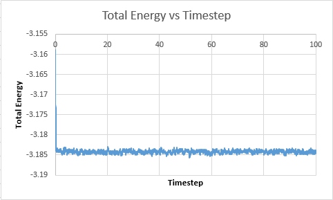

Temperature vs Timestep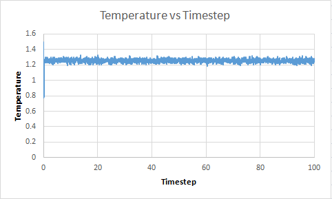

Pressure vs Timestep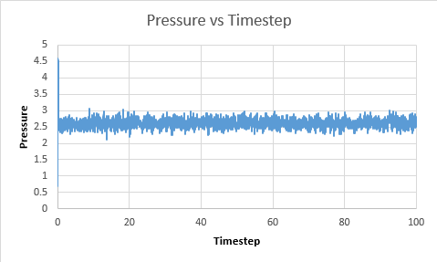

Total energy of all timesteps vs Timestep

The system does reach equilibrium after a few timesteps.The largest timestep value to give accetable results is 0.0025. This is because it reaches the same equilibrium value of 0.001, however it requires less overall time to achieve this and so is a better timestep. For timestep of value 0.015, it can be seen that the values diverge. This is because the time between readings is so large. According to the Velocity verlet theorum, it takes the previous position and velocity of the particle. As the particle may have moved a large distance from its previous position, without taking a measurement, there is a poor correlation between these two values and so the values diverge.

Running simulations under specific conditions

TASK: We need to choose $γ$ so that the temperature is correct $T = 𝔗$ if we multiply every velocity $γ$ . We can write two equations:

$\frac{1}{2} \sum_{i} m_{i} v_{i}^{2} = \frac{3}{2} N k_{B} T$

$\frac{1}{2} \sum_{i} m_{i} {(γ v_{i})}^{2} = \frac{3}{2} N k_{B} 𝔗$

Solve these to determine $γ$ .

$γ = (\frac{3 N k_{B} 𝔗}{\sum_{i} m_{i} v_{i}^{2}})^{1 / 2}$

TASK: Use the manual page to find out the importance of the three numbers 100 1000 100000. How often will values of the temperature, etc., be sampled for the average? How many measurements contribute to the average? Looking to the following line, how much time will you simulate?

100 represents after how many timesteps to take an average of the results. ${A_{v}}_{n} = \frac{\sum_{i} T i m e s t e p s}{100}$

1000 after all the averages have been made, what to average it by again. $N_{i} = \frac{\sum_{i} A_{v} 1 + A_{v} 2 + A_{v n} . . .}{1000}$

10,000 represents after averaging the 1000 averages and left with one average, what to average it by again. $A_{a} = \frac{\sum_{i} N_{i}}{10000}$

This is averages of averages

TASK: When your simulations have finished, download the log files as before. At the end of the log file, LAMMPS will output the values and errors for the pressure, temperature, and density $(\frac{N}{V})$ . Use software of your choice to plot the density as a function of temperature for both of the pressures that you simulated. Your graph(s) should include error bars in both the x and y directions. You should also include a line corresponding to the density predicted by the ideal gas law at that pressure. Is your simulated density lower or higher? Justify this. Does the discrepancy increase or decrease with pressure?

Total energy vs Timestep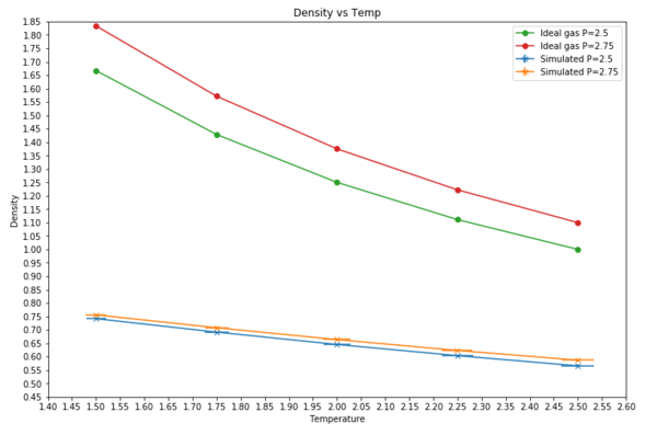

Simulated density lower because for ideal gas molecules, they do not interact and so the Leonard jones potential is not active. This means for the ideal gas there no repulsive term. When molecules close to each other, repulsive term dominates and as it is not active, the molecules can get as close as possible increasing the overall density. The discrepancy decreases with increased temperature.

Calculating heat capacities using statistical physics

TASK: As in the last section, you need to run simulations at ten phase points. In this section, we will be in density-temperature $(ρ^{*}, T^{*})$ phase space, rather than pressure-temperature phase space. The two densities required at $0.2$ and $0.8$ , and the temperature range is $2.0, 2.2, 2.4, 2.6, 2.8$ . Plot $C_{V} / V$ as a function of temperature, where $V$ is the volume of the simulation cell, for both of your densities (on the same graph). Is the trend the one you would expect? Attach an example of one of your input scripts to your report.

Cv/V vs Temperature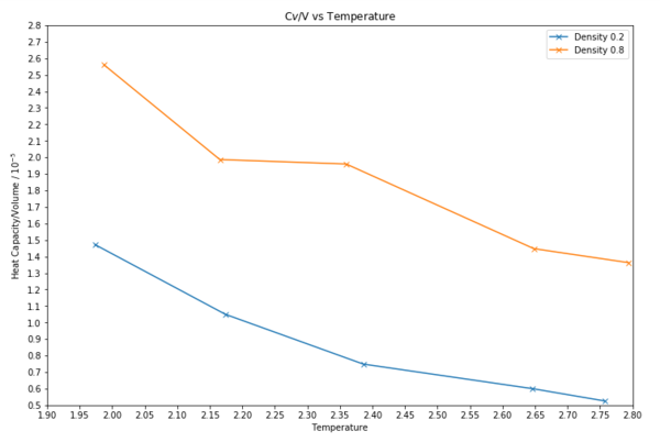

The trend is what I would expect. There is a higher density for a constant number of particles. A large variance value correlates to a large heat capacity as the energy states are close together. This means the accessibility of energy levels is higher and thus means that the energy states are more likely to be populated overall meaning a higher heat capacity.

Find attached the input script for the temperature and pressure of 0.2,2.0 from this address

Structural properties and the radial distribution function

TASK: perform simulations of the Lennard-Jones system in the three phases. When each is complete, download the trajectory and calculate $g (r)$ and $\int g (r) d r$ . Plot the RDFs for the three systems on the same axes, and attach a copy to your report. Discuss qualitatively the differences between the three RDFs, and what this tells you about the structure of the system in each phase. In the solid case, illustrate which lattice sites the first three peaks correspond to. What is the lattice spacing? What is the coordination number for each of the first three peaks?

g(r) vs Timestep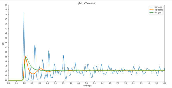

Integral g(r) vs Timestep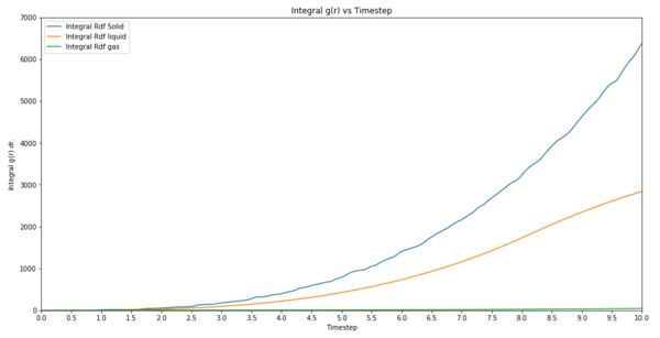

g(r) is a measure of the probability of finding a particle at a distance of r away from a given particle, in comparison to that for an ideal gas. It can be seen from the plots that the differences between the RDFs are that the gas rdf converges to a value much faster than the other two. This means that the system density quickly becomes uniform. For a liquid density of atoms converge to the same value but it takes longer than gas. As for a solid, it takes a lot longer. This tells us that because a gas can quickly have a uniform density throughout the system, its structure is not uniform. This means a solid is confined and does not have much thermal energy it takes much longer for density to equilibrate. The first three peaks are due to the face centred lattice sites. The lattice spacing is 1.38672 per side. Coordination number of 12.

Dynamical properties and the diffusion coefficient

TASK: make a plot for each of your simulations (solid, liquid, and gas), showing the mean squared displacement (the "total" MSD) as a function of timestep. Are these as you would expect? Estimate $D$ in each case. Be careful with the units! Repeat this procedure for the MSD data that you were given from the one million atom simulations.

Mean squared displacement vs Timestep

Millon atoms mean squared displacement vs Timestep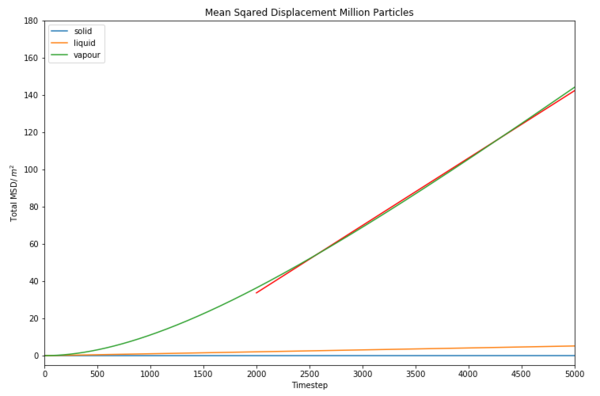

Mean squared displacement measures the deviation time between the position of a particle and some reference position. For vapour it would be very high as the distance each particle deviates from its initial position is large as it has high kinetic energy. This therefore means the value of D will be large in comparison to liquid and solid.

Solid value of $D = 1.4404129119349059 * 1 0^{- 9} m^{2}$

Liquid value of $D = 0.0001697955150048799 m^{2}$

Gas value of $D = 0.012052181893094415 m^{2}$

For million particles

Solid value of $D = 8.7825979277857917 * 1 0^{- 9} m^{2}$

Liquid value of $D = 0.00017452860832099627 m^{2}$

Gas value of $D = 0.0060319737644783907 m^{2}$

It can also be seen for a larger number of molecules the value of D decreases, this is because the system is now greatly populated than before meaning it is harder for the atoms to move past other atoms, and so its displacement is reduced.

Molecular dynamics simulations of simple liquids

Abstract

This research shows the capabilities computational chemistry can accomplish with modelling complex systems. Different thermodynamic quantities can be and are calculated ranging from temperature of the system to the diffusion coefficient with high accuracy. By modelling different systems it has been shown that approximations like the ideal gas law are incomparable to real life results. These models bring insight and reproducible results in the real world.

Introduction

Computer simulations are used everyday for a variety of reasons such as calculating molecular reaction quantities, bond vibrations, bond lengths, Gibbs free energy etc. They give real life solutions without having to conduct a physical experiment, saving time and resources.Comparing computed measurements to real life measurements and getting them as close as possible means that we are able to then visually understand how molecules behave by simulating a series of steps. For this simulation understanding the motion of liquids is conducted. A liquid is a defined as a substance that takes the form of the container it is placed in. There are a variety of liquids that exist with a variety of properties that define it such as surface tension, intermolecular interactions, volatility. Water is a strange liquid and is still widely examined because of its unusual properties, for example it's intermolecular bonding. Because oxygen is a very electronegative atom in comparison to hydrogen, water is capable of forming hydrogen bonding which has a great impact on its physical properties such as boiling temperature and freezing point. Hydrogen bonds are very strong and so the energy required to break these bonds is very high. Because of hydrogen bonding, ice has a strange property such that ice can float on water. This is unlike any other solids, for the solid form to be less dense than the liquid. During the freezing process because there is not enough kinetic energy for hydrogen bonds to be broken, the water molecules align to form a lattice structure with the molecules further apart than in a liquid state arising to an overall lower density.

Aims and Objectives

The aims of this simulation was to understand how to simulate liquids of only one particle type, setting their physical properties and their interactions via the Leonard jones interaction. It was also to obtain an output of the thermodynamic properties of the system such as average temperature, pressure, volume, energy, density, heat capacity, rdf, mean squared displacement and the diffusion coefficient. Thereby seeing how changing temperature and density affects these quantities.

Methodology

Positions and velocities were calculated using the Verlet Algorithm and Velocity Verlet Algorithm. For the velocity verlet theorem, you can calculate a (1/2) timestep with the same accuracy of a single timestep however you require your previous position and velocity. The value of the timestep was determined by testing variable timesteps and seeing what the lowest value you could achieve before having the system reach equilibrium. In all the physical properties of atoms section standard conditions included the mass, pair_style and pair_coeff were defined. Mass was given a type of 1 and mass of 1.0, type 1 defining the properties of that specific atom. Pair_style lj/cut/opt 3.0 was used, defining the Leonard Jones pairwise interactions. Pair_coeff 1 1 1.0 1.0 describes the pairwise force field coefficients between two type 1 atoms.

Simulations under specific conditions

The simulation box geometry section was to define the lattice type and size. Sc 0.8 was used generating a simple cubic lattice with one lattice point per cell. The value 0.8 describes the number of lattice points per unit volume. This then generates a box length 1.07722 (in reduced units) in each direction. The lattice is expanded to a region of size 15 by 15 by 15, generating 3375 atoms. 5 temperatures and 2 pressures were selected and 10 different simulations were run. The temperatures selected were 1.5, 1.75, 2.0, 2.25, 2.5 and pressures selected were 2.5 and 2.75. The velocities of atoms in any system were distributed using the Maxwell-Boltzmann distribution. The number of particles, volume and total energy were all fixed. Output values included time, total energy, temperature and pressure. The density was then plotted as a function of temperature for both of the pressures that were simulated.

Calculating heat capacities using statistical physics

Sc 0.8 and 0.2 was used. A density of 0.2 generates a cube with each size equaling 1.70998. The lattice is expanded to a region of size 15 by 15 by 15, generating 3375 atoms. 5 temperatures were selected, 10 different simulations were run. The temperatures selected were 2.0,2.2,2.4,2.6,2.8. The velocities of atoms in any system were distributed using the Maxwell-Boltzmann distribution. The system was brought to the desired state using unfix nvt fix nve all nve. Output values included time, total energy, temperature, density, number of atoms and volume. A plot $\frac{C_{v}}{V}$ as a function of temperature was made by finding heat capacity using the equation:

$C_{V} = N^{2} \frac{⟨ E^{2} ⟩ - {⟨ E ⟩}^{2}}{k_{B} T^{2}}$ ^[1]

Structural properties and the radial distribution function

Three phases were assessed for the rdf function by assessing a density temperature phase diagram and locating the values which corrispond to a solid, liquid and gas.^[2] For a solid, Fcc 1.5 and temperature 0.2 was used, generating a face centered cubic lattice with 4 lattice points. This lattice is expanded to a region of size 15 by 15 by 15, generating 13500 atoms. The velocities of atoms in any system were distributed using the Maxwell-Boltzmann distribution. The simulation was run for 10,000 timesteps. g(r) was then computed using the trajectories in the software VMD. The data was then plotted against timesteps.

Dynamical properties and the diffusion coefficient

Three phases were assessed for the diffusion coefficient. For a solid, Fcc 1.5 and temperature 0.2 was used. This lattice is expanded to a region of size 15 by 15 by 15, generating 13500 atoms. For a liquid sc 0.8 and temperature 1.2 was used. For a gas sc 0.01 and temperature 1.0 was used. The velocities of atoms in any system were distributed using the Maxwell-Boltzmann distribution. The simulation was run for 10,000 timesteps. To measure D it was required to measure the mean squared displacement with the equation $D = \frac{1}{6} \frac{\partial ⟨ r^{2} (t) ⟩}{\partial t}$ ^[1] A plot was made for each simulation showing the mean squared displacement as a function of timestep. D was then estimated from the linear region gradient of each graph. This was then repeated for the msd data of million atoms.

Results and discussion

For simulations under specific conditions, it was found that the density of the simulated runs were lower than the ideal gas projections. This is because in the simulated runs, the Leonard Jones force field is active and so when the atoms are close to each other the repulsive term dominates and so the density is low. In comparison, for an ideal gas there are no Leonard Jones interactions and so atoms can approach each other as close as they possibly can, making the density higher. This is supported by the graph showing that for both pressures and temperature ranges, the ideal gas plot is at a higher density value and the error bars observed are miniscule.

For calculating heat capacities using statistical physics, it was found that the heat capacity of a more dense system is higher. A large value in $⟨ E^{2} ⟩ - {⟨ E ⟩}^{2}$ correlates to a large heat capacity. This is because the energy states of they whole system are close together. This means the accessibility of energy levels is higher and thus means that the energy states are more likely to be populated, overall meaning a higher heat capacity. This is supported by the plot as the plot with a density of 0.8 has a higher value overall and so has a higher heat capacity.

For structural properties and the radial distribution function it was found that the gas converges to a value of 1.0 faster than a liquid or solid meaning that the system density quickly becomes uniform. This is seen by the difference in shapes of the graphs where the solid plot fluctuates greatly compared to liquid and gas. The reason why a gas converges faster is because the molecules have a greater capability to move around and so are able to evenly distribute itself in the container whereas a solid is rigid and so it can only vibrate. It takes much longer for a solid then to reach an equilibrium.

For dynamical properties and the diffusion coefficient, it was found that the gas diffusion was very high in comparison to the liquid and solid at a value of 0.012052181893094415. Similarly for the million particle version of this experiment, the gas has the highest value at 0.0060319737644783907 . This is because a gas molecule has more kinetic energy than a solid or a liquid. This means that the atom is able to move a greater distance from its starting position than a solid or liquid would. This is supported by the large gradient on the graph compared to the very small solid and liquid gradients which are approximately equal to zero. It can also be seen for a larger number of molecules the value of D decreases, this is because the system is now greatly populated than before meaning it is harder for the atoms to move past other atoms, and so its displacement is reduced.

Conclusion

It was shown how particles of a single type interact in different phases and conditions. To expand understanding of how liquids behave, including molecules of different masses could be implemented. Also, terms to include a molecules polarity could help us understand further how water interacts with itself and other molecules at varying temperatures and pressures.

References

↑ ^1.0 ^1.1 Professor Fernando Bresme. Third year simulation experiment. Available: https://wiki.ch.ic.ac.uk/wiki/index.php?title=Third_year_simulation_experiment. Last accessed 25/10/2017
↑ Cite error: Invalid <ref> tag; no text was provided for refs named Paper page

[Wiki_page-1] 1.0 ^1.1 Professor Fernando Bresme. Third year simulation experiment. Available: https://wiki.ch.ic.ac.uk/wiki/index.php?title=Third_year_simulation_experiment. Last accessed 25/10/2017

[Paper_page-2] Cite error: Invalid <ref> tag; no text was provided for refs named Paper page

[1]

[2]