Rep:DSB113

Completing Harmonic Oscillator

The Velocity-Verlet algorithm is used to model the behaviour of a classical harmonic oscillator.

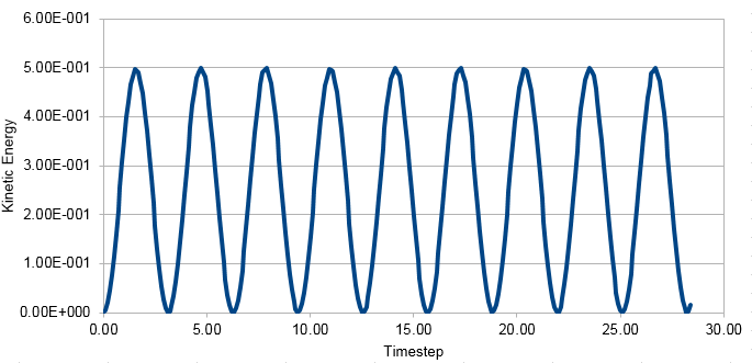
Energy in this case was just kinetic energy not total energy. Potential energy was added to this using the formula  Φ= 0.5kx^2, where k is the force constant and x is distance.

Calculation Parameters

Φ	0.00
A	1.00
ω	1.00
mass	1.00
k	1.00
original timestep	0.1
updated timestep	0.2

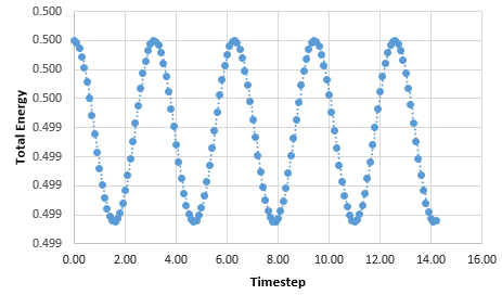
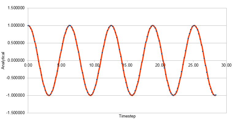
The position of maxima in error were estimated and plotted against time generating the formula; y = 0.0004x- 7E-05. The timestep was varied to provide an error within 1%. The timestep used was 0.2, as increasing the timestep increased the error. The original timestep used through the Harmonic Oscillator model was 0.1. This reduced the error. It is important to monitor the total energy of a physical system to ensure energy is conserved and to see any changes.

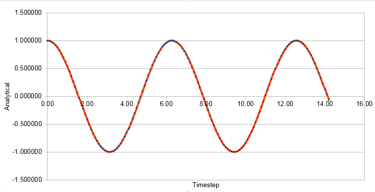
Graph showing the Analytical solution against timestep

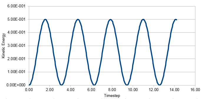
Graph showing the Kinetic Energy against timestep

Graph showing the error against timestep

Graph showing the maximum error against timestep

Graph showing the total energy against timestep

The graphs above are for a timestep of 0.1. The graphs below show an increase in timestep to 0.2 providing an error within 1%.

Graph showing the Analytical solution against timestep when timestep has been doubled from 0.1 to 0.2

Graph showing the Kinetic Energy against timestep when timestep has been doubled from 0.1 to 0.2

Graph showing the error against timestep when timestep has been doubled from 0.1 to 0.2 to ensure error is only 1%

Lennard-Jones Interaction

When the potential energy is zero, the formula rearranges to show that r₀=σ.

The force at this separation is calculated by differentiating to give

Periodic Boundary Conditions

Realistic volumes of liquid cannot be simulated due to the number of water particles involved as shown below.

The number of water molecules in 1ml of water under standard conditions is calculated using density of water and Avagadros Number. 1ml=1g, 1/18 (Molar mass of water) x 6.022 x 10²³ =3.34 x 10²².

The volume of 10000 water molecules is calculated by doing the reverse of above. 10000/(6.022 x 10²³) = 1.66 x 10^-20. This is the number of Moles of 10000 water molecules. Multiply this by 18 to find the mass of 10000 water molecules which is 3 x 10^-19 g converted to cm³ is the same as density of water is 1 g/cm³.

If an atom at position (0.5, 0.5, 0.5) moves along vector (0.7, 0.6, 0.2) it ends up at (0.2, 0.1, 0.7) after periodic boundary conditions have been applied.

The Lennard-Jones parameter for argon are σ=0.34nm ε/K_B=120K.

If the cutoff is 3.2, r is 1.088 in real units as r*= r/σ.

The well depth is 1.656 x 10^-21 as ε/K_B=120K where ε is the well depth and K_B is the Boltzmann constant.

Similarly if the reduced temperature (T*) is 1.5, T is 180K in real units as T* = (k_BT)/ ε

Creating the Simulation Box

As there is no order a single point of reference cannot be used to find positions of all other atoms in liquid and vapour phases.

Giving atoms random starting coordinates causes problems in simulations as atoms may land on top of each other and repel causing minor explosions.

If the distance between points of a lattice are 1.07722 in reduced units, the number density of a 0.8

1 lattice point. 

For a face-centred cubic lattice, with a number density of 1.2, the side length of the cubic unit cell is 1.36 in reduced units. Through the create_atoms command, 3000 atoms would be created if this lattice had been defined.

Setting the Properties of the atoms

The purpose of:

mass 1 1.0

is to define the mass of atom type 1 which is 1.0

pair_style lj/cut 3.0

is defining the Lennard-Jones cutoff as 3.0 with no coulomb interaction.

pair_coeff ** 1.0 1.0

defines that for each type of atom and each other type of atom, the interaction remains the same at 1.0.

Since both x_i (0) and v_i (0) are being specified, the Velocity-Verlet algorithm will be used.

The reason just 

timestep 0.001

run 100000

is not written is due to the fact that the timestep being used numerous times. Using the other method makes it easier to change timesteps and hence easier to compare the results. 

Checking Equilibration 

It is of paramount importance that the system reaches equilibrium state.

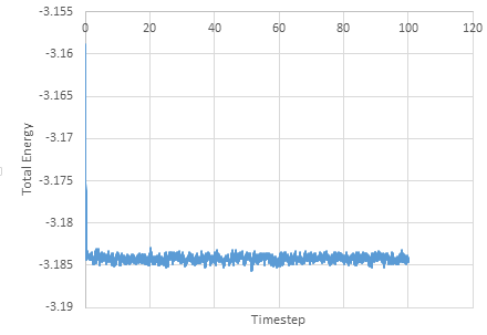
Graph showing the Total Energy against timestep

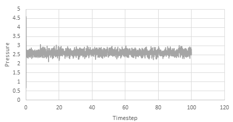
Graph showing the Pressure against timestep

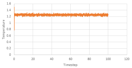
Graph showing the Temperature against timestep

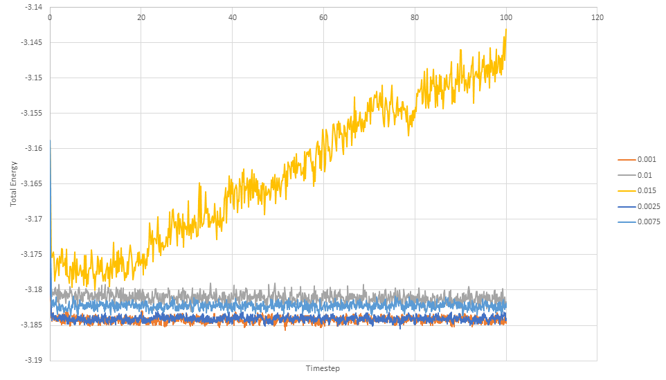
Graph showing the Total Energy against timestep at individual timesteps

The simulation reaches equilibrium at 0.41. A timestep of 0.01 is the largest to give acceptable results. The 0.015 timestep is a particularly bad choice as the simulation doesn't reach equilibrium. The energy of this time step decreases initially before increasing rapidly. 

Temperature and Pressure Control

The systme upto this point was run under a microconical ensemble. Now the system will be run under isobaric-isothermal ensemble. The timestep used for this is 0.0075

Temperature	Pressure 1	Pressure 2
1.6	2.6	3.5
2.0	2.6	3.5
2.4	2.6	3.5
2.8	2.6	3.5
3.2	2.6	3.5

As T fluctuates, a constant factor is used to ensure the target temperature is achieved. If temperature is higher than target, the constant is less than 1 however, if the target is higher than the temperature the constant is greater than 1. Using these 2 equations:

by dividing the first equation from the second equation, it can be seen that $\gamma =\sqrt{\left(\frac{\mathfrak{𝔗}}{T}\right)}$

If the ave setting is window, then the values produced on timesteps that are multiples of Nfreq are summed and averaged within a moving “window” of time, so that the last M values are used to produce the output. E.g. if M = 3 and Nfreq = 1000, then the output on step 10000 will be the average of the individual values on steps 8000,9000,10000. Outputs on early steps will average over less than M values if they are not available.

Values of temperature will be sampled every 100 units for the average. 1000 measurements contribute to the average. Since the timestep used in this case is 0.0075 and there are 1000 measurements, the time simulated will be 7.5

Plotting Equations of State

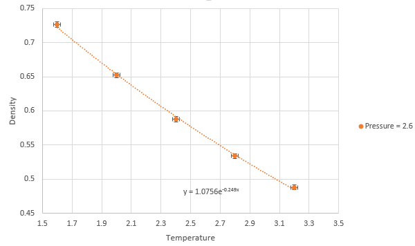
Graph showing density against temperature at pressure of 2.6 with error bars

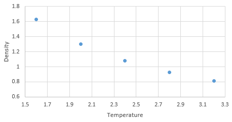
Graph showing density against temperature using the ideal gas law at pressure of 2.6

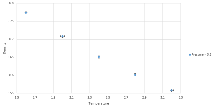
Graph showing density against temperature at pressure of 3.5 with error bars

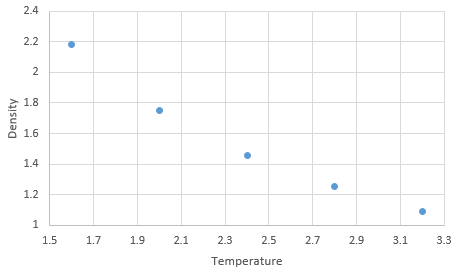
Graph showing density against temperature using the ideal gas law at pressure of 3.5

The simulated density using the ideal gas law simulates higher densities at both pressures due to assumptions made under the law. The ideal gas law doesn't account for molecular size or intermolecular interactions. As temperature increases, the effect of intermolecular interactions decreases. As pressure increases the discrepancy increases.

Calculating Heat Capacity

In thermodynamics, many uantities can be calculated by considering how much the system can fluctuate from its average equilibrium state.

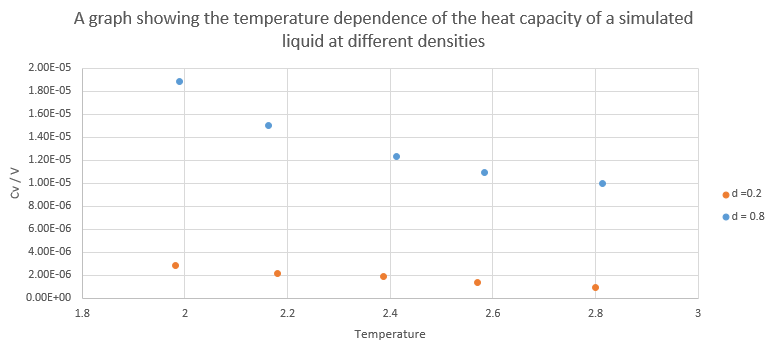
Graph showing Heat capacity/volume against temperature at density of 0.2 and 0.8

A copy of an example input script can be found here Media:d8t28.ogg. This is an example when density is 0.8 and Temperature is 2.8.

At both densities, the heat capacity/volume decreases as temperature increases. Lower density has lower heat capacity as heat capacity is an intensive property.

Radial Distribution Function

The RDF provides the distance between an atom and its nearest neighbour, second nearest, etc. It can be found experimentally hence ensures the simulation is reproducing correctly. The atomic trajectory is recorded to generate the RDF.

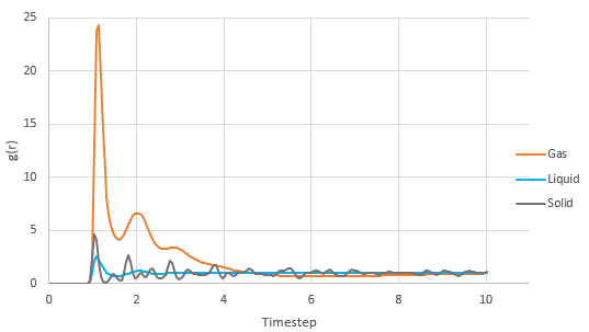
Graph showing the Radial Distribution Function denoted by g(r) of the 3 phases against timestep

Graph showing the integrated radial distribution function of the 3 phases against timestep

FCC lattice representation

The RDF shows the distance between x from the centre of the atom and the probability. A gas phase has very few neighboring atoms as the RDF shows the fewest peaks while solid has the most neighboring atoms and hence the most peaks. The first 3 peaks correspond to the 4 atoms closest to the atom being observed, followed by the atom in a similar position but 1 up and finally another 4 atoms which are 1.5 up. Peaks 1 and 3 correspond to 4 atoms as the atoms are equidistant from the atom being observed. The lattice spacing is 0.8 in reduced units calculated by finding the difference between 2 maximas which correspond to 0.5 of the hypotenuse.The coordination number for each of the first 3 peaks is 12, 18 and 42 respectively. This is found by looking at the first 3 minimas after a peak on g(r) and finding the equivalent timestep and hence the integrated g(r) value.

Mean Squared Displacement

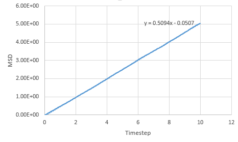
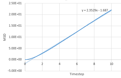
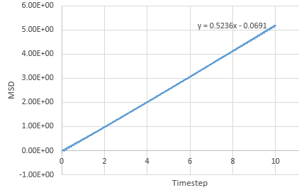
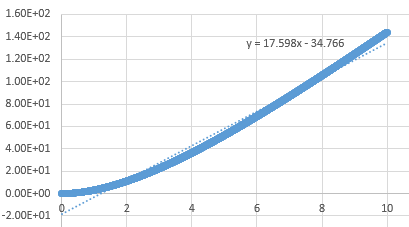
The MSD provides information on how much atoms in the simulation move around, characterised by the diffucsion coefficient.

Graph showing the mean squared displacement against timestep for a liquid

Graph showing the mean squared displacement against timestep for a solid

Graph showing the mean squared displacement against timestep for a vapour

Graph showing the mean squared displacement against timestep for a liquid for a million particles

Graph showing the mean squared displacement against timestep for a solid for a million particles

Graph showing the mean squared displacement against timestep for a vapour for a million particles

The estimated D for liquid is 0.0849 reduced units, for solid its 0.0000005 reduced units and for vapour, its 0.39215 reduced units. The general trend observed is what is expected. A solid is tightly packed so will not move much however, a vapour is loosely packed and hence has the highest D. Increasing the number of particles to a million has very little effect on the Solid and liquid where D remains near the same, 0.000005 and 0.08726. However there is a large difference for the vapour phase which has D of 2.933 reduced units.

Velocity Autocorrelation Function

The diffusion coefficient can also be calculated using VACF which provides the difference in velocity between 2 different times. Velocities should not be correlated at long times indicating velocity is random.

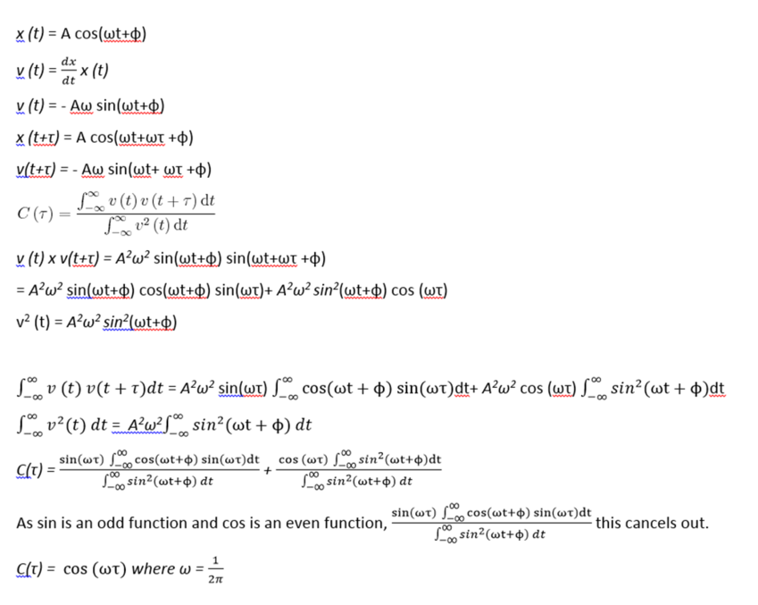
Graph showing the 1D harmonic oscillator function of the Velocity Autocorrelation Function denoted by C(t)

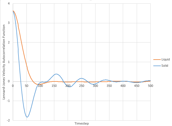
Lennard-Jones liquid and solid harmonic oscillator VACF.

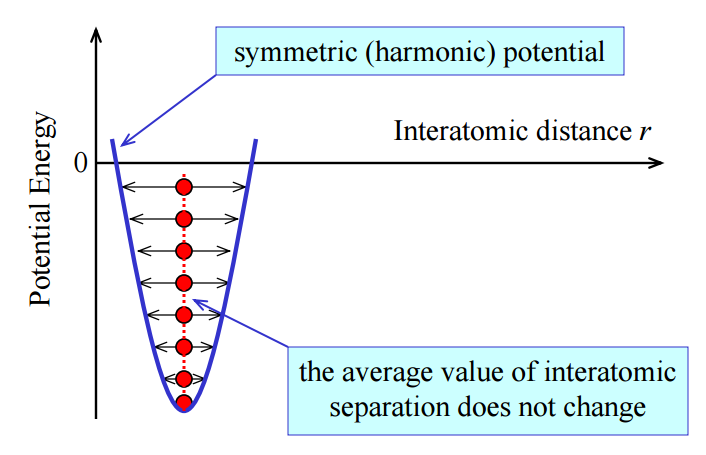
The minima in the VACFs for liquid and solid system represents the repulsion between atoms as the repulsive forces are stronger when the atoms are closer together. At the maxima, the atoms are moving in the same direction as there is a strong correlation. The difference between the liquid and solid is that liquid particles are able to move more compared to solid particles, this dampens the VACF as liquid particles have weaker inter-particle interactions. The harmonic oscillator is different to the Lennard Jones solid and liquid as the harmonic oscillator is not driven or damped. LJ solid and liquid account for friction/damping which slows the motion of the system by decreasing the velocity.

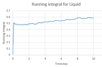
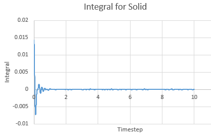
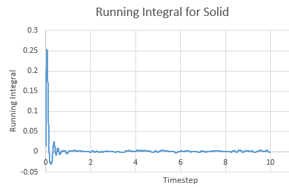
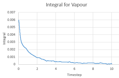
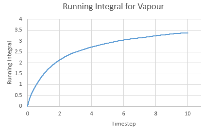
Phase	Running Integral	Diffusion Coefficient
Gas	3.382857	1.127619
Liquid	0.587281	0.19576
Solid	-0.00111	-0.00037

Integral for a liquid against timestep

Running Integral for a liquid against timestep

Integral for a solid against timestep

Running Integral for a solid against timestep

Integral for a vapour against timestep

Running Integral for a vapour against timestep

The Integral was calculated using the trapezium rule. The largest source of error is decreasing the size of each trapezium to increase the accuracy.