Rep:DL3715LiquidSimulation

Overall: An ok report - you need to work on your style a bit. Your reports going into your final year project need to be more in line with what you read in literature and less what you expect we (the markers) expect (which isn't what we do expect ironically!). Rather than explaining background theory (which is good for you to understand, but if the reader needs to understand it it's the readers prerogative to pick up a book!) explain the research background. All introductions you write shold be literature surveys and deliver some interesting relevant research that provdes your work with worth. Anyway, good effort. Mark: 65/100

Abstract

Not a bad abstract but I would include data - remember the abstract is a really short, concise summary of your work's purpose, important data (here diffusion coefficients for both msd and vacf) and take home messages. Simulations of Lennard-Jones solid, liquid and vapour were run under different ensembles through LAMMPS on the Imperial HPC service. The effect of temperature and pressure on heat capacity was investigated by simulations on the grand canonical ensemble we run simulations under ensembles on systems - the ensemble isn't so much the system but more properties we're defining constant. The structure of the solid, liquid and vapour phase of argon were studied by the radial distribution functions. we didn't study argon, we studied lennard-jones fluid, although comparable! The first three coordination sphere of argon in the solid state was observed from the integrated radial distribution functions. The dynamic properties of the system were illustrated by the mean squared displacement . In particular, the calculated self- diffusion coefficient from the velocity autocorrelation function by integration using trapezium rule was compared to the results from the gradient of the mean squared displacement. In addition, the effect of atom counts on simulations was explored by comparing results getting from a simple 1000 atoms system and that of a one million atoms system. Limitations and main source of error were discussed. The evaluation of the normalised velocity autocorrelation function was solved from the First Principle.Not sure I would call it first principle but certainly derived for the harmonic oscillator

Introduction

Good that you understand things but this is quite an unrefined introduction. Before your MSci/BSc project, you need to get out of this habit of explaining background theory and highlight the background here. Where is this research in the grand scheme of things? Who has worked on it? How is this applied? https://doi.org/10.4271/932811 is a really good paper presenting an application for diffusion/dynamic based phase research and talking about this in your introduction will hook mechanical engineers to your work (this is an example - you could talk about this sort of research in any context!). If you don't provide a niche, nobody cares!

Material state is characterised by the spacing between neighbouring atoms: solid has a regular spacing, neighbours can be found at characteristic distances; liquid has a irregular spacing with neighbours found at approximate distances; whereas gas has a more irregular spacing, the distances between neighbours are less defined.Think less about spacing and more about systematic ordering

Diffusion usually not usually, it does! takes place from a region of high concentration to one of low concentration. Once the system reaches a uniform concentration, the process of molecular diffusion is determined by the process of self- diffusion. The diffusion coefficient depends largely on the density of the system. Study of the diffusion coefficient is important for understanding the chemical reaction as well as phase transformations.

In quantum chemistry, the Schrodinger equation is a good model for describing hydrogen atom based chemical systems. For systems containing other atoms than hydrogen, approximations have to be made. The classical particle approximation assumes all atoms behave classically so each of them interact with all the rest. If we want to measure a physical property of a system, we need to sum that physical property for each individual atoms. Computer simulation becomes useful when modelling a collection of atoms for a system. Verlet algorithm solves the calculation by breaking the simulation rather than continuous functions of time, but as a sequence of timesteps. For example, when calculating the total force of a system, the position of the atoms at each timesteps are calculated. From the Newton's second law as shown below (Eqn. 1), the force at each timesteps are calculated but no velocity information.

$$\begin{gathered} {\mathbf{F}}_i=m_i\frac{{\mathrm{d}}^2{\mathbf{x}}_i}{\mathrm{d}{t}^2} \\ (Eqn.1) \end{gathered}$$

Velocity Verlet algorithm incorporates velocity, solving the first-timestep problem in the Verlet algorithm. In particular, positions and velocities can be computed by integrating the equations of motion (Eqn. 1) using half-time-step velocities. However, the initial condition of the system about the position and velocity of the atoms must be chosen at the beginning of the simulation.

By classical physics, the force experienced by each molecule is obtained from its potential energy:

$$\begin{gathered} {\mathbf{F}}_i=-\frac{\mathrm{d}U\left({\mathbf{r}}^N\right)}{\mathrm{d}{\mathbf{r}}_i} \\ (Eqn.2) \end{gathered}$$

where rⁿ is the net force vector on the molecule and r is the position vector of the molecule. Thus, the potential energy is essentially dependent on the position of the molecule. Lennard-Jones pair potential (Eqn.3) is considered to be a good model for the interactions between pairs of atoms.

$$\begin{gathered} U\left({\mathbf{r}}^N\right)=\sum _i^N\sum _{i\ne j}^N\left\{4ϵ(\frac{{\sigma }^{12}}{r_{ij}^{12}}-\frac{{\sigma }^6}{r_{ij}^6})\right\} \\ (Eqn.3) \end{gathered}$$

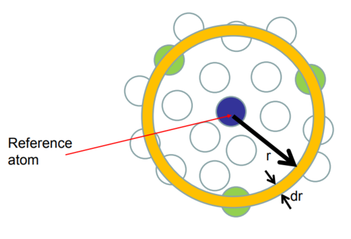
In a simulation, the atoms are initially placed in a regular lattice with an initial displacement. The forces acting on each atom in the ensemble are then computed and the resulting motion or change in the motion calculated for each atom by solving the equations of motion. After a short timestep, the new positions are calculated, then the new forces and the change in motions, etc. The system is taken to be at equilibrium when the initial impulse is dissipated throughout the system and the temperature or energy of the system is reasonable stable. Radial Distribution Function (RDF) describes how on average atoms are radially packed in a system. It is a particularly effective way of describing the structure of disordered molecular systems like liquids. In liquids, there is continual movement of the atoms and a single snapshot of the system shows only the instantaneous disorder.

Aims and Objectives

This lab is aimed to introduce how to run a simulation by LAMMPS and more importantly, how to extract useful experimental data from the output of the simulation by manipulating fundamental equations and data analysis from chosen software.

A good computational methods section sticks to a structure - model, parameters, forcefield, parameters, tools. This sort of section needs some work and joined dialogue :)

Methods

All simulations were run on the Imperial College HPC facility performed with LAMMPS runtime option. All graphs and respective data were produced and analysed using Excel.

Running first simulations

The first five simulations with five different timesteps of 0.001, 0.0025, 0.0075, 0.01, 0.015 were edited in textfile based on the given melt_crystal.in file in the Intro folder. The edited five simulation files were performed with LAMMPS on HPC. The output file was analysed in Excel from row 25.

Visualising the trajectory

The trajectory files were visualised in VMD programme. The Sphere Scale was set to 0.3 and the Sphere Resolution was set to 17. The Drawing method in the Graphics Representations were changed from Lines to Points. By clicking Create Rep, index 1 or index 2 was entered in the Selected Atoms box to track a single particle.

Temperature and Pressure Control

Ten simulations at temperature 2,4,6,8,10 and pressure at 1.8 and 2.5 were created based on the file npt.in and then submitted to the HPC portal. Data was output as log files.

Heat Capacity Calculation

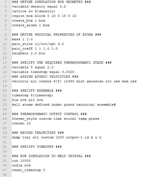
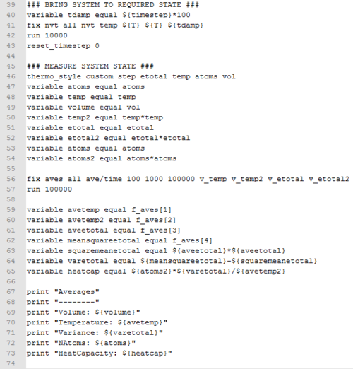
Ten simulations at temperature 2.0, 2.2, 2.4, 2.6, 2.8, and densities at 0.2 and 0.8 were submitted to the HPC portal. Data was output as log files. The input script is shown below.

Fig.1. the input script for heat capacity calculation (1)

Fig.2. the input script for heat capacity calculation (2)

Radial Distribution Function

The simulations of the Lennard-Jones system of in the three phases (solid (fcc): density = 1.5, temp = 1.15; Liquid: density = 0.606, temp = 1.15; Gas:density = 0.073, temp = 1.15;) were performed on the HPC. The output data was saved as the trajectory file. In VMD, the interested trajectory was loaded. By choosing the Analysis in the Extensions folder, the Radial Pair Distribution Function g(r) was selected to display g(r) and Int(g(r)). The computed plots were saved and analysed in Excel.

Dynamic Properties and the Diffusion Coefficient

Three simulations with specified density and temperature (solid: density = 1.5, temp = 1.15; Liquid: density = 0.606, temp = 1.15; Gas:density = 0.073, temp = 1.15;) were run to calculate the mean squared displacement and velocity autocorrelation function. The 'optional output-2' data file was saved. The procedure was repeated for the system of one million atoms.

Results and Discussion

All the TASK problems were discussed and underlines in this section, following the order as in the script.

Velocity Verlet Algorithm

In the file HO.xls.In, the 'Analytical' was calculated by the position of a classical harmonic oscillator given by x (t) = A cos (ωt + Φ) [ A = 1, ω = 1, Φ = 0 ].

'Error' was given by the absolute difference between the 'Velocity Verlet solution' and the 'Analytical' solution.

'Energy' was the sum of the kinetic and potential energy of the oscillator for the velocity verlet solution.

At the default timestep value of 0.1, the positions of the maxima in the error were estimated and plotted as a function of time in orange as shown in Fig.3.The equation of line of best fit was shown on the graph. The error in the Velocity Verlet solution was building up in the course of the simulation.

Fig.3. the maxima in error as a function of time

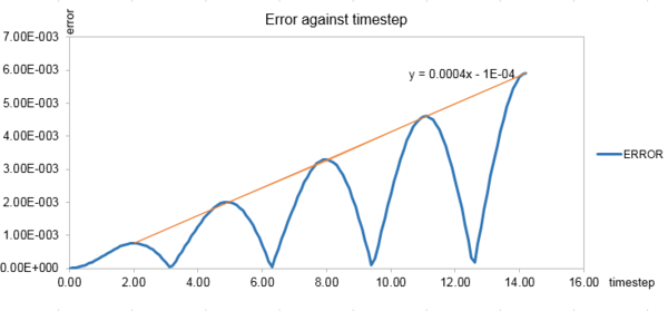
The maximum and minimum limits of the energy (fluctuation within 1% of total energy) were plotted in blue and orange in Fig. 2. Timesteps from 0.1 to 0.3 were tested. The energy was kept within the allowed fluctuation limit until the timestep was greater than 0.2 as shown below in grey. Thus, a timestep of 0.2 gave the lowest average relative percentage error with shortest average computer time.tick

Fig.4. the energy plot at timestep=0.2

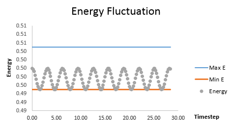
It is important to monitor the total energy of a physical system when modelling its behaviour because the fluctuation in energy can cause an increase in the error of the Velocity Verlet solution (when the timestep was increased to 0.3, the error was significantly larger).

Atomic Forces

For a single Lennard-Jones interaction, at potential energy equals zero, the separation r₀ is the crossing point of the curve with x-axis at σ (r₀ = σ).The atom experiences a repulsion force of 2.394 ε / σ at that separation of σ since the σ¹²/r¹² term dominates in the Lennard-Jones potential. The equilibrium separation r _eq is the minimum point in the potential well and the well depth Φ (r_eq) is the minimum potential point ε ($r_{eq}=2^{1/6}\sigma$).

$\frac{d\varphi (r)}{dr}=24ϵ(\frac{2{\sigma }^{12}}{r^{13}}-\frac{1{\sigma }^6}{r^7})=0$ $\frac{2{\sigma }^{12}}{r^{13}}=\frac{{\sigma }^6}{r^7}$ $2{\sigma }^6=r^6$ $r_{eq}=2^{1/6}\sigma$

tick

Three sets of potential energies were calculated from the integration of Eqn.3 with three sets of limits of r (σ = ε = 1) as shown in the table below.

$\underset{2\sigma }{\overset{\mathrm{\infty }}{\int }}\varphi \left(r\right)\mathrm{d}r=4ϵ\underset{2\sigma }{\overset{\mathrm{\infty }}{\int }}(\frac{{\sigma }^{12}}{r^{12}}-\frac{{\sigma }^6}{r^6})\mathrm{d}r$ $=4ϵ[\frac{{\sigma }^{12}}{-11r^{11}}+\frac{{\sigma }^6}{5r^5}{]}_{2\sigma }^{\mathrm{\infty }}$

Limit (r)	Integral
2σ - ∞	-0.0248
2.5σ - ∞	-0.00818
3σ - ∞	-0.00329

tick

By observation, the potential energy decreases as the distance between a pair of atoms increases. Beyond r = 3σ, we can safely ignore the barely exist interaction when doing simulation. We are only interested in the atomic interaction within this cutoff range (0 - 3σ). Under standard conditions, water has a density of 1 g/cm³. The mass of 1 mL water is 1 g and the molar mass of water is 18 g so 1/18 mole water molecule is present. By Avogadro's number (N_A = 6.022 ^ 10²³), there are 3.34 ^ 10²² water molecules in 1 mL of water under standard conditions.

10000 water molecules is 1.66 ^ 10^-20 mole of water molecules. Thus, it has a mass of 2.99 ^ 10^-19 g (1.66 ^ 10^-20 ^ 18). According to v = m / d, the volume of 10000 water molecules is thus 2.99 ^ 10^-19 cm^-3 or 2.99 ^ 10^-25 m^-3.

Calculations are carried out in reduced units when working with Lennard-Jones for convenience. For argon, the conversion between the reduced units and real units is shown in the table below.

Parameter	Reduced units*	Real units
r	3.2	1.09 nm
ε	-	-0.997 KJ/mol-1
T	1.5	180 K

When an atom leaves the box, it is replaced by an atom coming in from the opposite side of the box with the same velocity (periodic boundary conditions). This avoids any effect of confinements on the dynamics. An atom at position (0.5, 0.5, 0.5) in a cubic simulation box which runs from (0, 0, 0) to (1, 1, 1). In a single timestep, it moves along the vector (1, 1, 1). After the periodic boundary conditions, it will be bounced back from the boundary around the box and end up at (0.2, 0.1, 0.7).tick

Equilibration

First, we assign atoms to vertices of the lattice to set a separation between atoms. This will avoid atoms overlapping with each other causing simulation blow-up (large repulsive forces and extremely high energy).

In a simple cubic lattice, there is one lattice point per unit cell. When the number density of lattice points is 0.8, the side length is 1.07722. When we have a face-centred cubic lattice with a lattice point number density of 1.2, the side length of the cubic unit cell can be calculated by l=³√N/ρ (N=4 lattice points per fcc unit cell) giving 1.49 in reduced unit.

The following lines in the input file defines the simulation box geometry so creates atoms at each lattice point.

region box block 0 10 0 10 0 10
create_box 1 box
create_atoms 1 box

According to the lines above, 1000 unit cells are created. Fcc lattice have four lattice points per unit cell so 4000 lattice points would be created if the lattice has a structure of fcc.

Next, the physical properties of atoms are defined as below.

mass 1 1.0
pair_style lj/cut 3.0
pair_coeff * * 1.0 1.0

Atoms of type 1 and mass 1 (hydrogen) are created in the box. According to to the LAMMPS manual, pair potentials are defined between pairs of atoms that are within a cutoff distance of 3 in reduced units ( 3σ in real unit, as discussed in the 'Atomic Force' section). Then, the atomic velocity is specified as below.

velocity all create 1.5 12345 dist gaussian rot yes mom yes

Since we are specifying x(0) and v(0), we are using the Velocity Verlet algorithm. All atoms created will be set in a 'create' style which generates an ensemble of velocities using a random number generator at specified temperature, 1.5, in reduced unit, but the velocity generated overall follows the Maxwell-Boltzmann distribution. The mom word and rot word are used under the create style. In this cases, it means the angular momentum is zeroed and the linear momentum of the newly created ensemble of velocities is zeroed. The dist gaussian word is also used under create. The ensemble of generated velocities will be a Gaussian distribution with a mean of 0.0 and a to product the requested temperature in reduced unit.

### SPECIFY TIMESTEP ###
variable timestep equal 0.001
variable n_steps equal floor(100/${timestep})
timestep ${timestep}

### RUN SIMULATION ###
run ${n_steps}
run 100000

The second line and third line in the above input file defines timestep as the variable. Instead of setting the timestep as 0.001, the timestep variable in the above format can be easily reset in the simulation.

Fig.5. the energy plot at timestep=0.001

Fig.6. the temperature plot at timestep=0.001

Fig.7. the pressure plot at timestep=0.001

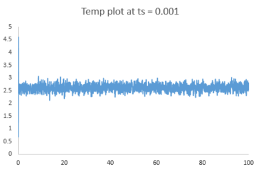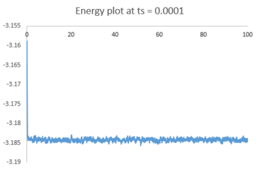
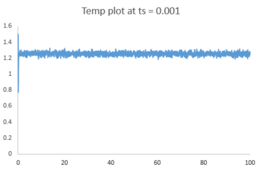
The plots of energy, temperature and pressure against time for the 0.001 timestep experiment are shown above. The simulation reaches equilibrium at about t = 0.35 (almost instantly).

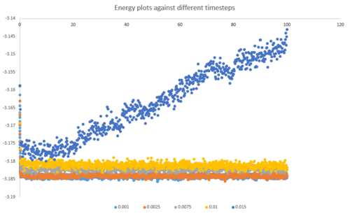
Below is a combined energy plot against time at various timesteps. It shows that at a timestep of 0.015, the simulation deviates from equilibrium. It is a bad choice of timestep because the timestep is too large to include all the essential details about the system and errors also accumulate in the course of simulation, resulting in the severe deviation. At timestep of 0.001 and 0.0025, the results getting from the simulation are almost equivalent in terms of the amount of details. Thus, the timestep of 0.0025 is the largest timestep (takes shorter time to simulate) that gives acceptable results.tick

Fig.8. the energy plot at various timesteps

Temperature and Pressure Control

By looking at the average pressure of the first set of simulations, temperature at 2, 4, 6, 8, and 10 in reduced unit and pressure at 1.8 and 2.5 in reduced unit were chosen to give 10 phase points. The optimum timestep of 0.0025 were chosen to run the 10 simulations.

The temperature of the simulation was controlled by a constant factor, $\gamma$. By equipartition theorem, in our system with N atoms, each with 3 degrees of freedom, the kinetic energy will be equal to $E_K=\frac{3}{2}N{k}_{B}T$.

At the end of every timestep, the instantaneous temperature T is calculation from the kinetics energy (1/2 ∑ mv² = 3/2 N K_B T) and it fluctuates slightly compared to our target temperature, $\mathfrak{𝔗}$. $\gamma <1$ was determined so that the instantaneous temperature is equal to the target temperature.

$$\begin{gathered} \frac{1}{2}\sum _i{m}_i{\gamma }^2 \\ {v}_i^2=\frac{3}{2}N{k}_B\mathfrak{𝔗} \end{gathered}$$

$$\begin{gathered} \frac{1}{2}\sum _i{m}_i \\ {v}_i^2=\frac{3}{2{\gamma }^2}N{k}_B\mathfrak{𝔗} \end{gathered}$$

$\frac{3}{2}N{k}_{B}T=\frac{3}{2{\gamma }^2}N{k}_B\mathfrak{𝔗}$ (since $$\begin{gathered} \frac{3}{2}N{k}_{B}T=\frac{1}{2}\sum _i{m}_i \\ {v}_i^2 \end{gathered}$$)

$\gamma =\sqrt{\frac{\mathfrak{𝔗}}{T}}$tick

The three numbers 100 1000 100000 in the below input file represent that values on timesteps of 100, 200, 300, ... , 900, 1000 are used to compute the final average on timestep 1000. (Nevery = 100, Nrepeat = 1000, Nfreq = 100000). The total simulation time will be 100000 * 0.0025 = 250 in reduced unit.

### MEASURE SYSTEM STATE ###
thermo_style custom step etotal temp press density
variable dens equal density
variable dens2 equal density*density
variable temp equal temp
variable temp2 equal temp*temp
variable press equal press
variable press2 equal press*press
fix aves all ave/time 100 1000 100000 v_dens v_temp v_press v_dens2 v_temp2 v_press2
run 100000

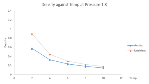
The density from the output log files was plotted as a function of temperature for both pressure at 1.8 and 2.5 as shown below (Fig.9 and 10). The error bars in x and y directions are presented on the graph. The density predicted by the ideal gas law (PV=nRT) was plotted on the graph as well.

Fig.9. the density plot at pressure = 1.8

Fig.10. the density plot at pressure = 2.5

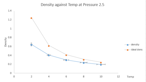The simulated density is always lower than the ideal density and this discrepancy increases with pressure. The ideal density assumes there is no interatomic interaction. However, in our Lennard-Jones system, repulsion force dominates over attraction between atoms. Thus, atoms are further away compared to the ideal gas situation. Larger volume is occupied so in general, the simulated density is lower than the ideal density. At higher temperature, atoms move faster so further away from each other. From Lennard-Jones equation (Eqn.3), the attraction term starts to take over the repulsion, therefore, the interaction is more an ideal behaviour. The discrepancy at higher temperature is smaller. Similar to the temperature effect, at higher pressure, atoms collide more frequently and the interaction between atoms leads to a greater deviation from ideal gas behaviour.tick, good

Heat Capacity Calculation

Another 10 sets of simulations were submitted to investigate the trend in heat capacity as a function of temperature.

In the input file, the properties of the box was firstly defined as a simple cubic lattice with density of 0.2 and creating 15*15*15 unit cells in total. All the unit cells are filled with type 1 atoms (hydrogen).

variable density equal 0.2
lattice sc ${density}
region box block 0 15 0 15 0 15
create_box 1 box
create_atoms 1 box

All the physical properties of atoms and the required thermodynamic state are specified as before. Besides, the ensemble we are using this time has a different property compared to the previous temperature and pressure constant system. All atoms are defined under the grand canonical ensemble as below.

### SPECIFY ENSEMBLE ###
timestep ${timestep}
fix nve all nve

The heat capacity is measured by the fluctuation in the total energy of the system and is calculated by the equation below (Eqn. 4).

$$\begin{gathered} C_V=N^2\frac{⟨E^2⟩-{⟨E⟩}^2}{k_B{T}^2} \\ (Eqn.4) \end{gathered}$$

Thus, in the input file, the heat capacity is defined as the number of atoms squared multiplied by the variance of the energy and divided by the temperature squared as shown in the bottom line of the input file below.

### MEASURE SYSTEM STATE ###
thermo_style custom step etotal temp atoms vol
variable atoms equal atoms
variable temp equal temp
variable volume equal vol
variable temp2 equal temp*temp
variable etotal equal etotal
variable etotal2 equal etotal*etotal
variable atoms equal atoms
variable atoms2 equal atoms*atoms

fix aves all ave/time 100 1000 100000 v_temp v_temp2 v_etotal v_etotal2 
run 100000

variable avetemp equal f_aves[1]
variable avetemp2 equal f_aves[2]
variable aveetotal equal f_aves[3]
variable meansquareetotal equal f_aves[4]
variable squaremeanetotal equal ${aveetotal}*${aveetotal}
variable varetotal equal ${meansquareetotal}-${squaremeanetotal}
variable heatcap equal ${atoms2}*${varetotal}/${avetemp2}

The output file contains information about the volume, temperature, variance and heat capacity of the system. The heat capacity scaled by the volume of the simulated cell was plotted against temperature for both densities of 0.2 and 0.8 as shown in Fig.11.

Fig.11. the heat capacity against temperature plot at density 0.2 and 0.8

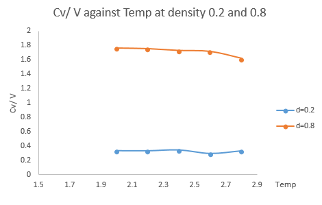
According to the theory about the density of states, it is easier to reach a higher state when the density of states is large. In the higher density system (d = 0.8), the heat capacity decreases as the temperature increases. At higher temperature, more states can be occupied at that energy level. High variance E means it is easier to populate high energy states. It takes less energy to promote all the atoms already at a higher energy state compared to all at the ground state. Thus, the heat capacity decreases as the temperature increases.

The discontinuity in the trend is observed at T = 2.6 for both systems. This fluctuation is likely due to a phase transition. The particles in the system are total symmetric. By equipartition theorem, the particle has no extra degree of freedom to reach, except from the only active translational mode, so it undergoes a phase transition. or we also dealing with a Lennard-Jones fluid thus there are no other degrees of freedom! If the density is not specified, melting will be seen as an access to more degree of freedoms. The volume of the system is constant throughout simulation, so the phase transition is unlikely to be a first ordered transition. Also, in a first order phase transition, the heat capacity tends to infinity at the transition point. In conclusion, the system undergoes a second order phase transition at T = 2.6 in reduced unit.

Although the same trend is less pronounced in the lower density system (d = 0.2), it will eventually decrease as the higher density system did if a larger simulation temperature range was chosen.

Structural properties and the radial distribution function

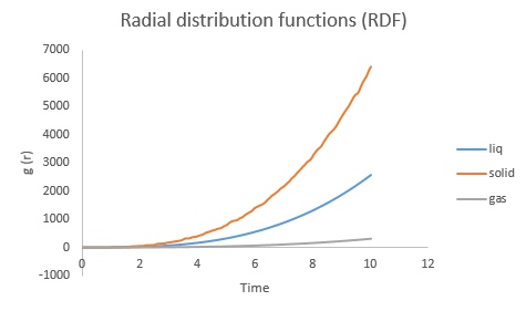
The RDF data was imported and analysed by Excel in Fig.12 and 13.

The density of a liquid only differed slightly from that of the corresponding solid hence the mean separation must be comparable in two states. The fundamental differences between the solid and liquid state of a material is the long range order in the crystalline solid and only a local order in liquid (shorter distance range).

Fig.12. the radial distribution functions in three phases

Fig.13. the integrated radial distribution functions in three phases

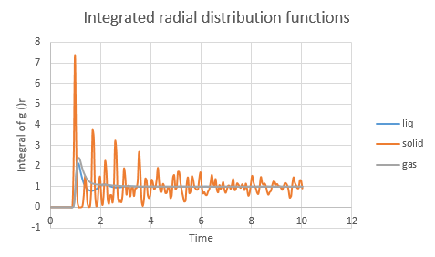The Radial Distribution Function is the ratio of density of atoms at distance r by overall density. In other words, it is the relative density of atoms as function of radius. Peaks in the RDF indicates a particularly favoured seperation distance for the neighbours to a given particle. The first peak corresponds to the nearest neighbour shell, the second peak to the second nearest neighbour shell, etc. Thus, RDF tells details about the atomic structure of the system being simulated. The number of atoms in the first coordination shell is about the same in liquid and solid but the two structures become quite different after the first coordination shell. For the liquid state, the initial peaks are likely to be the first and second solvation shells.

At all temperatures, the RDF of solid (at specific density) consists of discrete peaks (although peaks do broaden on temperature), which means the regularity of the lattice structure is always maintained during the simulation so there is no temperature at which the solid will melt.

Fig.14. illustration of radial distribution function

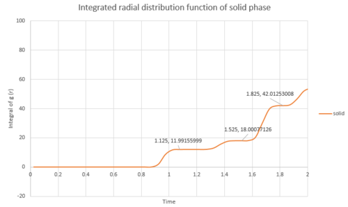
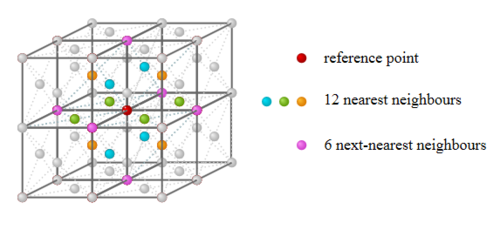
nice diagram For solid argon as shown in Fig.15, the first coordination shell contains 12 nearest neighbours, and additional 6 in the next shell, and extra 24 neighbours in the third coordination shell. Thus, it is arranged in a face centre cubic lattice. The arrangement of the neighbouring atoms in the first two coordination shells are shown in Fig.16.

Fig.15. the integrated radial distribution functions of solid phases

Fig.16. the first two coordination shells in a fcc lattice

Although RDF can provide information about dynamic change of structure, no information about how fast atoms move is provided.

Dynamic properties and the diffusion coefficient

One of the most important physical property of material is the diffusion coefficient which can be correlated to the mean squared displacement by Eqn. 5 shown below.

$$\begin{gathered} D=\frac{1}{6}\frac{1}{0.002}\frac{\partial ⟨r^2\left(t\right)⟩}{\partial t} \\ (Eqn.5) \end{gathered}$$

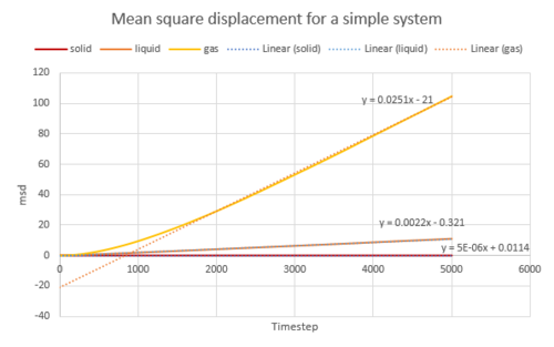
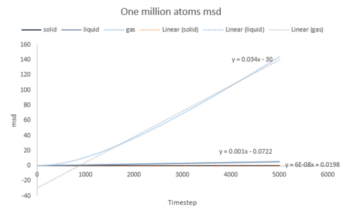
The diffusion coefficient was calculated from the gradient of the MSD plot for both the simple system and the one million atoms system. The data is shown in the table below and the plots are shown in Fig. 17, 18, 19.

	Diffusion Coefficient (simple system)	Diffusion Coefficient (one million atoms)
Solid	0.000417	0.000005
Liquid	0.183333	0.083333
Vapour	2.091667	2.833333

need units here! Look at your output file :)

Fig.17. the mean square displacement for a simple system

Fig.18. the mean square displacement for a million atoms

Fig.19. the plot of msd for both systems

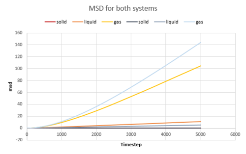The MSD is the highest for gas as they diffuse the quickest. The liquid has a larger MSD than solid. Solid atoms barely move at all, they vibrates around its position. The Velocity Autocorrelation Function was plotted in Fig. 20.

The results from one million atoms systems should be a better result on a larger atoms account.readability: on account that there are more atoms to sample The largest source of error comes from the integration by trapezium rule

Fig.20. the velocity autocorrelation for the liquid and solid systems

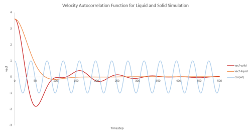
The autocorrelation function can be interpreted by dividing the graph into three regions.

The first part is the zero slope at time zero. At that instant, the atoms have a specific velocity of 3.6 in this simulation. If atoms in the system don't interact with each other, by Newton's Law of motion, the atoms would remain its velocity for all time. From our plot, the velocity is not a constant so there must be force acting on each other.

Backscattering effects of the atom from the shell of nearest neighbours results in a negative region of the velocity autocorrelation function¹. It becomes dominant in the higher density states (strong in solid state, weak in liquid state, not observed in vapour phase), where atoms are closely packed. In solid state, atoms are located where there is a near balance between repulsion and attraction forces. Atoms in high density states take longer to escape from its neighbourhood due to the reflection by neighbouring atoms. Therefore, their motion is a ballistic oscillation; the atoms reverse their velocity at the end of each oscillation. The resulted VAF oscillates strongly from positive to negative values with decaying magnitude. The $C\left(\tau \right)$ with $\omega =1/2\pi$ was plotted showing a perfect harmonic oscillation in ideal situation. There are perturbative forces acting on the atoms to disrupt the perfection of their oscillation. For example, the inelastic collision can cause a damped harmonic motion.

Liquids behave similarly to solids but without fixed regular positions. The oscillation between atoms is disturbed by the diffusion motion of liquid so the VAF decays faster to zero.

For gases, the backscattering effect completely disappears due to two reasons. Firstly, vapour atoms are too far to reflect each other. Secondly, the forces acting on the system have to increase for an increase in inelasticity if the system wants to achieve a stationary state of the same temperature. Long time-tail is observed with lower density states inelastic system. ²

The third region of decaying to zero shows the asymptotic behaviour which strongly depends on the density of the system. The smaller the density of state, the faster the system reaches the asymptotic decay.

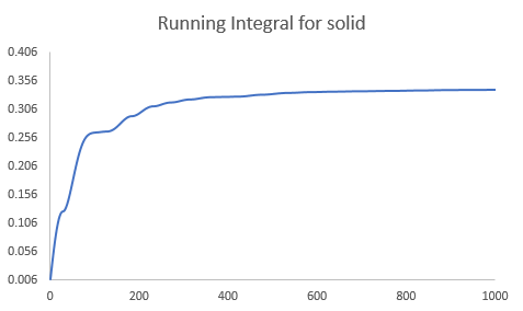
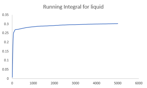
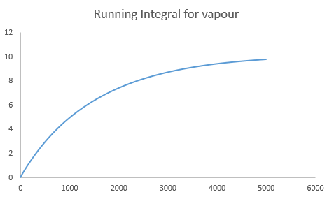
The diffusion coefficient can also be calculated from the integration of the velocity autocorrelation function by Eqn.6. The integration was carried out using the trapezium rule. The results obtained is shown below.

$$\begin{gathered} D=\frac{1}{3}\underset{0}{\overset{\mathrm{\infty }}{\int }}\mathrm{d}\tau ⟨\mathbf{v}\left(0\right)\cdot \mathbf{v}\left(\tau \right)⟩ \\ (Eqn.6) \end{gathered}$$

	Diffusion Coefficient (simple system)	Diffusion Coefficient (one million atoms)
Solid	0.000061	0.000046
Liquid	0.097897	0.090091
Vapour	3.353674	3.268421

Fig.21. the running integral for solid

Fig.22. the running integral for liquid

Fig.23. the running integral for vapour

The evaluation of the normalised velocity autocorrelation function for a 1D harmonic oscillator (Eqn.7) is shown below.

$$\begin{gathered} C\left(\tau \right)=\frac{\underset{-\mathrm{\infty }}{\overset{\mathrm{\infty }}{\int }}v\left(t\right)v(t+\tau )\mathrm{d}t}{\underset{-\mathrm{\infty }}{\overset{\mathrm{\infty }}{\int }}{v}^2\left(t\right)\mathrm{d}t} \\ (Eqn.7) \end{gathered}$$

Fig.24. the evaluation of the integral

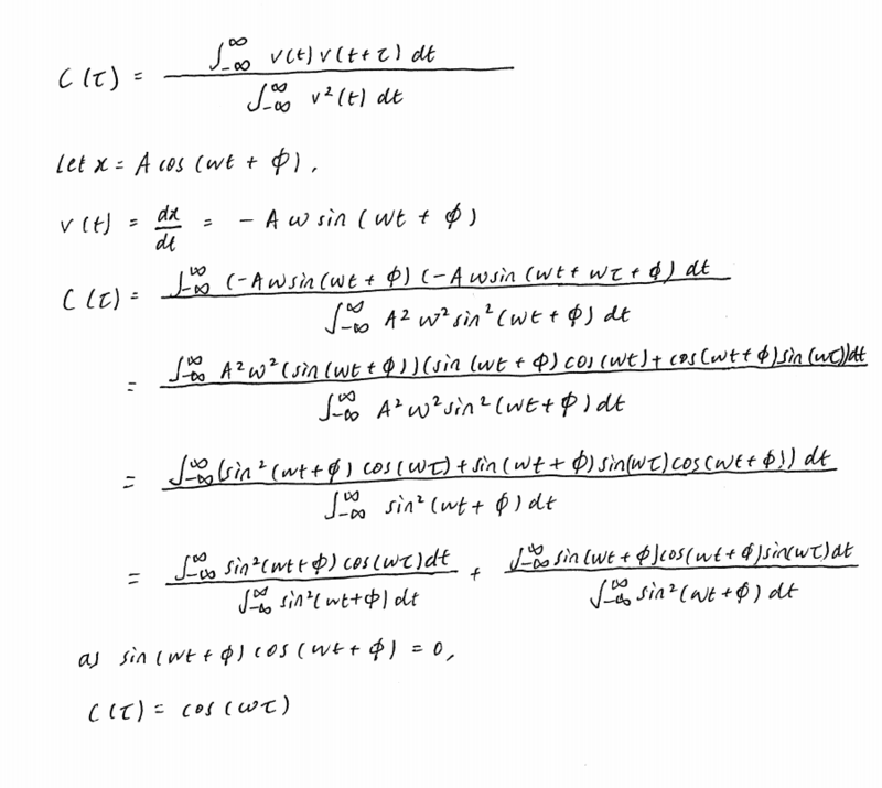
tick, good

Conclusion

Not bad but remember to tie the conclusion to the underlying theme of your work - this underlying theme must be presented in your introduction. The simulations of Lennard-Jones model of solid, liquid and vapour systems using the Velocity- Verlet algorithm were successfully carried out by LAMMPS. With a chosen timestep of 0.0025 in reduced unit, the system reached equilibrium instantly after the stimulation started. The error between the analytical solution and the Velocity-Verlet algorithm solution and the total energy of the system were monitored against time. The density of the system at constant temperature and pressure was plotted against time. By comparing the density obtained from simulation and from the ideal gas law, it is concluded that the repulsion force dominates in the Lennard- Jones model so the simulated density is always lower than the theoretical density of an ideal gas. Moreover, the decrease in heat capacity with the increase in temperature was reasoned by the density of states theory. The coordination number of a face centre cubic argon lattice was successfully determined from the integrated radial distribution function. Finally, the self- diffusion coefficient in three states was determined by integration of the velocity autocorrelation function by trapezium rule. The solid state has the smallest diffusion coefficient due to the ballistic oscillation in its lattice site, whereas vapour has the largest diffusion coefficient which concurs with the fact that vapours are always much more diffusive than liquids and solids.

References

1. R.A. Reis et al. / Fluid Phase Equilibria 221 (2004) 25–33

2. Int. J. Thermophys. 26: 1389-1407 (2005)