Rep:Cmpjp2916
Background
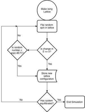
This experiment sets out to construct a programme to simulate a 2D Ising Lattice and to extract observable properties using Monte Carlo methods.
The Ising Model is a model of ferromagnetism where a material is reduced to a regular 2D lattice with spins restricted to two states. This greatly reduces the complexity of the problem while retaining the basic physics of a ferromagnetic material. The Hamiltonian for every spin site is , J represents the coupling constant between spin sites and determines the either ferromagnetic or anti-ferromagnetic nature of the lattice.
If further simplifications are made in the form of taking J to be unity, then the Boltzmann distribution function; gives the probability of finding the system is each possible state. This means the observables can be calculated simply by probability summing. This brings about computational challenges as there are 2^N possible configurations of an Ising Lattice, the practicalities of this are discussed later.
The solution to the above problem would be the reduction of the probability distribution of the infinite phase space to a representative distribution with a discrete number of points from the phase space. The Mertropolis method generates successive states from theirs predecessors through a valid transition probability. This method proves successful in allowing a random sample of the probability distribution and is what enables the use of Monte Carlo methods in the calculation of observables of the Ising Model.
Introduction to the Ising Model
TASK: Show that the lowest possible energy for the Ising model is , where is the number of dimensions and is the total number of spins. What is the multiplicity of this state? Calculate its entropy.
In a 1D lattice each spin has 2 neighbours, 2D spin has 4 etc. It follows that a spin has 2D neighbours, where D is the lattice dimension. Energy of the lattice is minimised when all spins are parallel; for all ; therefore the energy of this system is given by:
Entropy of a system is given by:
Multiplicity of the minimum energy spin system is 2, since there are two isoenergetic states where all spins are either up or down. Therefore the entropy of this system is:
TASK: Imagine that the system is in the lowest energy configuration. To move to a different state, one of the spins must spontaneously change direction ("flip"). What is the change in energy if this happens (D=3,\ N=1000)? How much entropy does the system gain by doing so?
The multiplicity of the new system is 2000, and so its entropy is .
TASK: Calculate the magnetisation of the 1D and 2D lattices in figure 1. What magnetisation would you expect to observe for an Ising lattice with D = 3,\ N=1000 at absolute zero?

1D: M = 1 2D: M = 1
3D at absolute zero, the system has access to the lowest energy configuration only where all spins are parallel. Therefore, M = ±1000.
Calculating the Energy and Magnetisation
TASK: complete the functions energy() and magnetisation(), which should return the energy of the lattice and the total magnetisation, respectively.
def energy(self):
     return -(np.sum(np.multiply(self.lattice,np.roll(self.lattice,1,1)))
+np.sum(np.multiply(self.lattice,np.roll(self.lattice,1,0))))

def magnetisation(self):
     return np.sum(self.lattice)
TASK: Run the ILcheck.py script from the IPython Qt console using the command

Introduction to the Monte Carlo Simulation
TASK: How many configurations are available to a system with 100 spins? To evaluate these expressions, we have to calculate the energy and magnetisation for each of these configurations, then perform the sum. Let's be very, very, generous, and say that we can analyse configurations per second with our computer. How long will it take to evaluate a single value of ?
2^100 = 1.27x10^30 configurations

1.27x10^30/10^9 = 1.27x10^21 s to compute

1.27x10^21 s = 4.02x10^13 years
TASK: Implement a single cycle of the above algorithm in the montecarlocycle(T) function. Complete the statistics() function.
    def montecarlostep(self, T):
        rand_i = np.random.randint(0,self.n_rows)  #Generate random coordinates for spin flip
        rand_j = np.random.randint(0,self.n_rows)

        self.lattice[rand_i][rand_j] *= -1         #Flip the spin at the random coordinates
        Ediff = self.energy() - self.cE        #Calculate energy difference between new and original lattice

        if Ediff < 0:                            #Accepting new configuration if energy is lowered
            self.cE = self.energy()

        else:
            if np.random.random() <= np.exp(-Ediff/T):        #Monte Carlo perturbation
                self.cE = self.energy()
            else:
                self.lattice[rand_i][rand_j] *= -1

        self.E.append(self.cE)         #Updating lattice variables
        self.n_cycles += 1
        self.cM = self.magnetisation()
        self.M.append(self.cM)
        return self.cE, self.cM
    def statistics(self, t):
        self.E2 = np.sum(np.array(self.E)**2)/self.n_cycles   #Mean of squares
        self.M2 = np.sum(np.array(self.M)**2)/self.n_cycles
        self.E = np.sum(self.E)/self.n_cycles                 #Mean
        self.M = np.sum(self.M)/self.n_cycles
        return self.E, self.E2, self.M, self.M2, self.n_cycles
TASK: If , do you expect a spontaneous magnetisation (i.e. do you expect)? When the state of the simulation appears to stop changing (when you have reached an equilibrium state), use the controls to export the output to PNG and attach this to your report. You should also include the output from your statistics() function.
At, the system does not have enough energy to access states with random spin configurations, therefore large regions of parallel spins are expected. At this point the entropic contribution to internal energy is insignificant therefore spins will align to reduce energy; magnetisation will not be equal to 0.
Figure 12 illustrates the output of ILanim.py, in this case a metastable state. The output of statistics() for this run is does not equal the end value which can be seen on graphs of energy and magnetisation. This is due to inclusion of the random starting configuration in the average. The motivation of the following exercise is to eliminate this error. The principle of this demonstration is the same for truly minimised states.
| statistics() output 8x8 T = 0.5 | |
|---|---|
| E | -78.5 |
| E^2 | 6560 |
| M | 8.60 |
| M^2 | 108 |

Accelerating the Code
TASK: Use the script ILtimetrial.py to record how long your current version of IsingLattice.py takes to perform 2000 Monte Carlo steps. This will vary, depending on what else the computer happens to be doing, so perform repeats and report the error in your average!
(When working through the lab I used the roll function to begin with, the energy() function below is one I wrote for this exercise. See below a run of ILcheck.py)

    def energy(self):
        e = 0
        for i in range(self.n_cols):
            e += np.sum(self.lattice[::,i-1]*self.lattice[::,i])
        for i in range(self.n_rows):
            e += np.sum(self.lattice[i-1,::]*self.lattice[i,::])
        return -e
| Run 1 | Run 2 | Run 3 | Run 4 | Run 5 | Average |
|---|---|---|---|---|---|
| 0.9450220000s | 0.9536990000s | 0.9670120000s | 0.9416790000s | 0.9676430000s | 0.9552s |
TASK: Use the script ILtimetrial.py to record how long your new version of IsingLattice.py takes to perform 2000 Monte Carlo steps. This will vary, depending on what else the computer happens to be doing, so perform repeats and report the error in your average!
| Run 1 | Run 2 | Run 3 | Run 4 | Run 5 | Average |
|---|---|---|---|---|---|
| 0.2485459999s | 0.2257899999s | 0.2320409999s | 0.2388259999s | 0.2355549999s | 0.2348s |
The Effect of Temperature
TASK: How many cycles are typically needed for the system to go from its random starting position to the equilibrium state? Modify your statistics() and montecarlostep() functions so that the first N cycles of the simulation are ignored when calculating the averages.
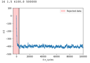
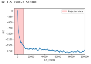
The script below determines the number of cycles required to reach equilibrium at the range of temperatures and lattice sizes which will be tested in later exercises. These 'parameters' are saved to a text file which is then imported by any other programmes which require the data. At the expense of a long wait to determine these parameters, any subsequent Monte Carlo simulations would be fast as there are no on the fly calculations of these parameters.
The script checks whether all spins are parallel or if the system has reached a metastable state characteristic of lattice sizes less than 10x10. The number of cycles to ignore when averaging is determined by finding the end of the sharp drop in energy of the random starting system after some Monte Carlo cycles.
While the method for finding the cut off point worked well; particularly for higher temperatures; but to achieve good average energies the simulations were ran for +500000 steps. Large systems at low temperatures would have difficulty reaching their minima, while smaller systems had a tendency to leave the minimum energy state and fluctuate only returning after considerable cycles.
For a full list of cut offs and runtimes please refer to the file below: Media:params.csv



from IsingLattice import *
import numpy as np

def end_state(model,fit):  #Tests for equilibration
    if (model.lattice == -1).all() or (model.lattice== 1).all():   #Parallel spins
        return False
    if (model.lattice== model.lattice[0]).all() or (model.lattice == np.vstack(model.lattice[:,0])).all(): #Metastable
        return False
    if model.n_cycles == 500000:
        return False

def eq_start(model):    #Determining cut off
    grad = []
    count = 0
    for i in range(100,model.n_cycles,100):   #Splitting energy data into chunks of 100
        grad += [np.std(model.E[i-100:i])]       #Standard deviation of data chunk
        if np.std(model.E[i-100:i]) > np.average(grad):     #Detects a change in gradient of the energy vs n_cycles curve
            count +=1
        if count == 3:  #Making a cut slightly later
            return i

    return model.n_cycles

ij = [2,4,8,16,32]
temps = np.linspace(0.25,5,39)
times = 3

data = np.empty((0,4))

for d in ij:
    for t in temps:
        cut = 0
        cycles = 0
        for i in range(times): #How many times to run simulation at given size and temperature
            fit = []
            il=IsingLattice(d,d)
            while end_state(il,fit) != False:  #Call end state test at every cycle
                il.montecarlostep(t)

            cut += eq_start(il)
            cycles += il.n_cycles*5
            print(d,t,cut/(1+i),il.n_cycles)
        data = np.vstack([data,[d,t,cut/times,cycles/times]]) #Save average cut and run time to the data array


print(data)
np.savetxt("params.csv", data)
import numpy as np

class IsingLattice:

    def __init__(self, n_rows, n_cols):
        self.n_rows = n_rows
        self.n_cols = n_cols
        self.lattice = np.random.choice([-1,1], size=(n_rows, n_cols))
        self.cE = self.energy()
        self.cM = self.magnetisation()
        self.E = [self.energy()]
        self.E2 = 0
        self.M = [self.magnetisation()]
        self.M2 = 0
        self.n_cycles = 0

        self.params = np.loadtxt('params.csv')[np.where(np.loadtxt('params.csv')[:,0] == [n_rows])[0]][:,1:]  #Load parameters file for specific lattice size only

    def energy(self):
        return -(np.sum(np.multiply(self.lattice,np.roll(self.lattice,1,1)))+np.sum(np.multiply(self.lattice,np.roll(self.lattice,1,0))))

    def magnetisation(self):
        return np.sum(self.lattice)

    def montecarlostep(self, T):
        rand_i = np.random.randint(0,self.n_rows)
        rand_j = np.random.randint(0,self.n_rows)

        self.lattice[rand_i][rand_j] *= -1
        Ediff = self.energy() - self.cE

        if Ediff < 0:
            self.cE = self.energy()

        else:
            if np.random.random() <= np.exp(-Ediff/T):
                self.cE = self.energy()
            else:
                self.lattice[rand_i][rand_j] *= -1

        self.E.append(self.cE)
        self.n_cycles += 1
        self.cM = self.magnetisation()
        self.M.append(self.cM)
        return self.cE, self.cM

    def statistics(self, t):  #Function now also takes temperature
        ave = int(self.params[np.where(self.params == t)[0]][0][1])    #Find cut off point for given temperature
        self.E2 = np.sum(np.array(self.E[ave:])**2)/(self.n_cycles-ave)
        self.M2 = np.sum(np.array(self.M[ave:])**2)/(self.n_cycles-ave)
        self.E = np.sum(self.E[ave:])/(self.n_cycles-ave)
        self.M = np.sum(self.M[ave:])/(self.n_cycles-ave)
        return self.E, self.E2, self.M, self.M2, self.n_cycles
The Effect of System Size
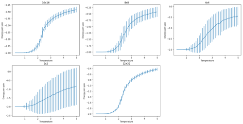
TASK: Repeat the final task of the previous section for the following lattice sizes: 2x2, 4x4, 8x8, 16x16, 32x32. How big a lattice do you think is big enough to capture the long range fluctuations?
The tendency of neighbouring spins to align will cause spontaneous magnetisation. Physically caused interactions between nearest neighbours propagating through the system. This means that the lattice can have net magnetisation in the absence of external magnetic field. This can be seen within the transition regions on the magnetisation curves. Where increasing lattice sizes show a smoother transition after their Curie temperatures. 16x16 is the largest lattice within which the jagged transition is seen and it can be expected that as lattice size tends towards infinity, this transition would be entirely smooth.

from IsingLattice import *
import glob
import pylab as plt
import numpy as np

#Copy of ILfinalframe.py as function

def temperaturerange(temps,times,n):
    il = IsingLattice(n,n)
    energies = []
    magnetisations = []
    energysq = []
    magnetisationsq = []

    ind = 0

    for t in temps:
        for i in times[ind]:
             energy, magnetisation = il.montecarlostep(t)

        aveE, aveE2, aveM, aveM2, n_cycles = il.statistics(t)
        energies.append(aveE)
        energysq.append(aveE2)
        magnetisations.append(aveM)
        magnetisationsq.append(aveM2)

        il.E = [il.energy()]
        il.E2 = 0
        il.M = [il.magnetisation()]
        il.M2 = 0
        il.n_cycles = 0
        ind += 1

    final_data = np.column_stack((temps, energies,
energysq, magnetisations, magnetisationsq))
    np.savetxt("{}x{}.dat".format(n,n), final_data)

dimensions = [2,4,8,16,32]
temps = np.linspace(0.25,5,39)
params = np.loadtxt('params.csv')[:,::3]

for n in dimensions:
    times = [range(int(i)) for i in params[np.where(params == n)[0],1]]  #Find runtime in params.csv
    temperaturerange(temps,times,n)

plt.subplots(figsize=(20, 10))
posi = (231)
spin = [16,8,4,2,32]
ind = 0

for filename in glob.glob('/Users/Jerzy/*.dat'):  #Plot graphs from .dat files
    data = np.genfromtxt(filename)
    err = np.sqrt(data[:,2]-data[:,1]**2)/spin[ind]**2  #Standard deviation from .dat
    plt.subplot(posi)
    plt.title('{}x{}'.format(spin[ind],spin[ind]))
    plt.xlabel('Temperature')
    plt.ylabel('Energy per spin')
    plt.errorbar(data[:,0],data[:,1]/spin[ind]**2,yerr = err)
    posi += 1
    ind += 1

plt.show()
Calculating the Heat Capacity
TASK: Write a Python script to make a plot showing the heat capacity versus temperature for each of your lattice sizes from the previous section.

import glob
import pylab as plt
import numpy as np

plt.subplots(figsize=(20, 10))
posi = (231)
spin = [16,8,4,2,32]
ind = 0

for filename in glob.glob('/Users/Jerzy/*.dat'):
    print(filename)
    data = np.genfromtxt(filename)
    var = data[:,2] - data[:,1]**2
    c = var/(data[:,0]**2)
    plt.subplot(posi)
    plt.title('{}x{}'.format(spin[ind],spin[ind]))
    plt.plot(data[:,0],c)
    plt.ylabel('Heat Capacity')
    plt.xlabel('Temperature')
    posi += 1
    ind += 1

plt.show()
Locating the Curie Temperature
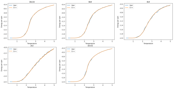
TASK: A C++ program has been used to run some much longer simulations than would be possible on the college computers in Python. For each lattice size, plot the C++ data against your data.
spin = [16,8,4,2,32] #bodge, order in which glob.glob spits out files
ind = 0
posi = (231)

plt.subplots(figsize=(20, 10))

for filename in glob.glob('/Users/Jerzy/Documents/Imperial/ImperialChem-Year3CMPExpt-master/C++_data/*.dat'): #Find all files in directory with .dat extension
    data = np.genfromtxt(filename)
    gendata = np.genfromtxt('/Users/Jerzy/{}'.format(filename[74:])) #Load user data for comparison
    plt.subplot(posi)
    plt.title('{}x{}'.format(spin[ind],spin[ind]))
    plt.xlabel('Temperature')
    plt.ylabel('Energy per spin')
    plt.plot(gendata[:,0],gendata[:,1]/spin[ind]**2,label = 'User')
    plt.plot(data[:,0],data[:,1],label = 'C++')
    plt.legend()
    ind += 1
    posi += 1

plt.show()
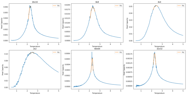
TASK: write a script to read the data from a particular file, and plot C vs T, as well as a fitted polynomial. Try changing the degree of the polynomial to improve the fit — in general, it might be difficult to get a good fit! Attach a PNG of an example fit to your report.

Increasing the order of polynomial does not improve the fit. It is likely that a very high order fit would give a curve resembling the date, yet the small fluctuations would introduce error when finding the peak heat capacity. The solution is to fit to data near the peak region with a low order polynomial; a smooth and accurate fit is achieved.
import glob
import pylab as plt
import numpy as np

def fit(data,peak):
    n = 12  #Range of data to include around peak
    fit = np.polyfit(data[peak-n:peak+n,0],data[peak-n:peak+n,-1],3) #Omitting data outside designated region, polynomial fit to data
    t_range = np.linspace(np.min(data[peak-n:peak+n,0]),np.max(data[peak-n:peak+n,0]),1000) #Creating temp data based on size of new range
    return np.polyval(fit,t_range), t_range #Polyval creates new y data based on fitted polynomial

spin = [16,8,4,2,64,32] #same fix
plt.subplots(figsize=(20,10))
posi = 231
ind = 0
curie = np.empty((0,2))

for filename in glob.glob('/Users/Jerzy/Documents/Imperial/ImperialChem-Year3CMPExpt-master/C++_data/*.dat'): #Load all .dat files in directiory
    data = np.genfromtxt(filename)
    peak = np.argmax(data[:,-1]) #Find maximum value of heat capacity
    fitc, fitt  = fit(data,peak)
    plt.subplot(posi)
    plt.title('{}x{}'.format(spin[ind],spin[ind]))
    plt.plot(data[:,0],data[:,-1])
    plt.plot(fitt, fitc,label= 'Fit')
    plt.legend()

    curie = np.vstack([curie,[spin[ind],fitt[np.where(fitc == np.max(fitc))]]])
    ind+=1
    posi += 1

plt.show()
np.savetxt('c++curie.dat',curie)
| Lattice Size | Curie Temperature |
|---|---|
| 2 | 2.51 |
| 4 | 2.44 |
| 8 | 2.33 |
| 16 | 2.32 |
| 32 | 2.29 |
| 64 | 2.28 |
TASK: Make a plot that uses the scaling relation given above to determine. By doing a little research online, you should be able to find the theoretical exact Curie temperature for the infinite 2D Ising lattice. How does your value compare to this? Are you surprised by how good/bad the agreement is?
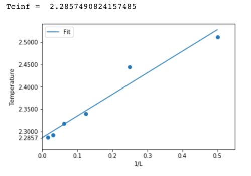
Plotting temperature against the inverse of lattice size yields the graph below. In accordance the the relationship , is found to be 2.29. This is a very small deviation from the theoretical value of 2.269. The most obvious source of error is the number of cycles for which the simulation was performed. As can be seen in figures 3 to 7, temperature fluctuations are high and therefore to achieve a good average many points must be considered.
