Rep:CMP 01180512 y3

Introduction to the Ising model

The Ising model consists of a rectangular lattice made up of discrete lattice sites with either +1 or -1 spins. These lattice sites experience periodic boundary conditions and interact with their immediate neighbours, in terms of exchange energy J. In a ferromagnetic model, adjacent parallel spins have favourable exchange energy while neighbouring antiparallel spins result in a higher energy state. This deceptively simple model should not be underestimated, due to its ability to predict phase transitions and thermodynamic properties of various phases of magnets. For instance, the beta-brass alloy can be modeled well with the Ising model, and the theoretical order-disorder transitions match experimental data obtained from x-ray scattering. More interestingly, the Ising model is used in neuroscience by Schneidman et. Al. to describe neuron activity as +1 (active) or -1 (inactive). The neuron activity of one axon influences the activity of another, sending a cascade of electrical signals in the brain.

In 1924, Lenz gave his student Ising the above model to solve , and Ising solved it for a 1D system. In 1944, Onsager provided a beautiful derivation for the 2D Ising model's partition function, which unlocked insights into the thermodynamic behaviour of the lattice. In this work, the 2D ising model would be simulated numerically using the Monte Carlo algorithm, and the various properties that emerge would be accounted for and compared to theoretical and literature results.

The model

Task 1

A. Show that the lowest possible energy for the Ising model is $$\begin{gathered} E \\ = \\ -DNJ \end{gathered}$$ where $D$ is the number of dimensions and $N$ is the total number of spins.

The Hamiltonian for the 2D Ising lattice is given byː

${\mathscr{H}}=-\frac{1}{2}J\sum _i^N\sum _{j\in \text{ neighbours }(i)}{s}_i{s}_j-E\sum _i{s}_i$

Where E is the external magnetic field that can point up or down and possess a magnitude. This is relevant in the context of Nuclear Magnetic Resonance (NMR) studies where spins interact with external magnetic fields. For the rest of the studies, a zero-field model is assumed for the sake of simplicity.

The total energy $E$ of the lattice in the absence of an external field is given by:

$$\begin{gathered} \begin{array}{rl}E& =-\frac{1}{2}J\sum _i^N\sum _{j \\ \in \\ \mathrm{n}\mathrm{e}\mathrm{i}\mathrm{g}\mathrm{h}\mathrm{b}\mathrm{o}\mathrm{u}\mathrm{r}\mathrm{s}\left(i\right)}{s}_i{s}_j\end{array} \end{gathered}$$

If the spins are aligned, $s_i{s}_j=+1$ and $E=-J$, if they are antiparallel, $s_i{s}_j=-1$ and $E=+J$.

Illustrations of 1D, 2D and 3D lattices with lattice sites of interest labeled.

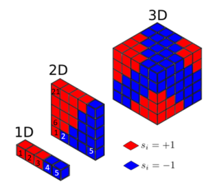
Looking at the 1D case with $N=5$, each lattice site interacts two times, with its left and right neighbours.

Assuming that all spins are aligned in the following calculations:

$\begin{array}{rl}E& =-J(s_1{s}_5+s_1{s}_2+s_2{s}_3+s_3{s}_4+s_4{s}_5)\\ & =-\frac{1}{2}J(s_1{s}_5+s_1{s}_2)\times 5\end{array}$

Note that if each atom is treated as having $2$ interactions, one might expect there to be $5\times 2$ for 5 lattice points. However, this would be double counting, since two neighbouring atoms have the same interactions with each other. A factor of $0.5$ is introduced to compensate.

Looking at the 2D case with $N=25$, each lattice site interacts four times, with its left, right, top and bottom neighbours

$\begin{array}{r}E=-\frac{1}{2}J(s_1{s}_2+s_1{s}_6+s_1{s}_{25}+s_1{s}_{25})\times 25\end{array}$

Looking at the $D$ Dimensional case with $N$ atoms, each lattice site interacts $2\times D$ times with its immediate neighbours. $0.5$ avoids double counting. The lowest possible energy $E$ occurs when all spins are aligned:

$\begin{array}{rl}E& =-\frac{1}{2}J(1\times 2D)\times N\\ & =-DNJ\end{array}$

B. What is the multiplicity of this state?

The multiplicity of this gound state can be represented with $\mathrm{\Omega }$. Since all the spin states are aligned, there are only two possible states: either all lattice points spin up or all spin down. These two states are degenerate in energy.

$\begin{array}{r}\mathrm{\Omega }=2\end{array}$

C. Calculate its entropy.

Entropy $S$ is defined as:

$\begin{array}{rl}S& =-k_B\ln \mathrm{\Omega }\end{array}$

Where $k_B$ is the Boltzmann constant.

For $\mathrm{\Omega }=2$:

$\begin{array}{rl}S& =k_B\ln 2\end{array}$

Phase Transitions

Task 2

A. Imagine that the system is in the lowest energy configuration. To move to a different state, one of the spins must spontaneously change direction ("flip"). What is the change in energy if this happens ($$\begin{gathered} D=3, \\ N=1000 \end{gathered}$$)?

The ground state for state of $$\begin{gathered} D=3, \\ N=1000 \end{gathered}$$ is given by $E_0$

$$\begin{gathered} \begin{array}{rl}E& =-\frac{1}{2}J\sum _i^N\sum _{j \\ \in \\ \mathrm{n}\mathrm{e}\mathrm{i}\mathrm{g}\mathrm{h}\mathrm{b}\mathrm{o}\mathrm{u}\mathrm{r}\mathrm{s}\left(i\right)}{s}_i{s}_j\\ E_0& =-\frac{1}{2}J(1\times 6)\times 1000\\ & =-3000J\end{array} \end{gathered}$$

If one state is flipped, there would be 6 formerly negative (energetically favouarble) $s_i{s}_j$ interactions becoming positive energy interactions instead. The energy would change from $-6J$ to $+6J$, representing an increasing of $12J$.

The new energy is given by:

$$\begin{gathered} \begin{array}{rl}{E}_{1 \\ flip}& =-3000J+12J\\ & =-2988J\end{array} \end{gathered}$$

B. How much entropy does the system gain by doing so?

If all spins in the lattice were initially +1, then the flip to -1 could happen for any particular lattice site out of the thousand. There are 1000 possible states with energetic degeneracy. If all spins were initially -1 instead, a flip will create another 1000 possible states. So in total, the number of microstates increased to $\mathrm{\Omega }=2000$ from $\mathrm{\Omega }=2$.

The change of entropy $=\mathrm{\Delta }S$ is given by:

$\begin{array}{rl}\mathrm{\Delta }S& =k_B\ln ({\mathrm{\Omega }}_{\text{new }}/{\mathrm{\Omega }}_{\text{old }})\\ & =k_B\ln \frac{2000}{2}\\ & =k_B\ln 1000\end{array}$

Task 3

A. Calculate the magnetisation of the 1D and 2D lattices in the figure below

The total magnetisation of the system $M$ is defined as:

$M=\sum _i{s}_i$

For a 1 D lattice:

$M=3-2=1$

For a 2 D lattice:

$M=13-12=1$

B. What magnetisation would you expect to observe for an Ising lattice with $$\begin{gathered} D=3, \\ N=1000 \end{gathered}$$ at absolute zero?

For 1000 spins, at 0 K, the Ising lattice would be at its ground state. This is because:

$F=U-TS$

When T=0 K, the free energy is determined solely by the exchange energy, which is at its lowest when all spins are aligned. The energy is lowest when the magnetisation is at its highest:

$M=1000$

Calculating the energy and Magnetisation

The final version of the code is available as: https://github.com/PanoptoSalad/Monte_Carlo_Ising_lattice/blob/main/IsingLattice_jiang.py

We can define our ising lattice as follows:

import numpy as np

class IsingLattice:

    E = 0.0
    E2 = 0.0
    M = 0.0
    M2 = 0.0

    n_cycles = 0

    def __init__(self, n_rows, n_cols):
        self.n_rows = n_rows
        self.n_cols = n_cols
        self.lattice = np.random.choice([-1,1], size=(n_rows, n_cols))

Task 1

Complete the functions energy() and magnetisation(), which should return the energy of the lattice and the total magnetisation, respectively. In the energy() function you may assume that $J=1.0$ at all times.

def energy(self):
    "Return the total energy of the current lattice configuration."
    N = self.n_cols * self.n_rows # Total number of spin states
    energy = 0.0
    for i in range(N):
        col = int(i % self.n_cols) # generate cols and rows with 1 for loop
        row = int((i - col) / self.n_cols) 
        energy += self.lattice[row][col] * self.lattice[row][col - 1] # interactions with left
        energy += self.lattice[row][col] * self.lattice[row - 1][col] # interactions with up
    return -energy

def magnetisation(self):
    "Return the total magnetisation of the current lattice configuration."
    magnetisation = np.sum(self.lattice) # adds up all the spin values in the lattice
    return magnetisation

Task 2

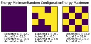
Run the ILcheck.py script from the IPython Qt console using the command

Results from the ILcheck.py script. The expected Energy, E and magnetisation, M calculated from the code written previously in this work matched values of the script

Introduction to the Monte Carlo simulation

Introduced in 1953, the Monte Carlo approach is a computational tour de force devised by Metropolis et Al. It is a stochastic method that aims to locate global minima by providing probabilistic perturbations to probe the energy surface. This allows the simulation to achieve ergodicity by overcoming potential barriers (provided temperature is high enough) and sample the whole configuration space of the lattice. It is a Markov chain process, whose future state depends entirely on its current state.

Algorithimic logic flow chart of Monte Carlo method to simulate Ising Lattice for a number of cycles

Average Energy and Magnetisation

Task 1

A. How many configurations are available to a system with 100 spins?

Each cell has 2 possible spin states, so with 100 cells, there are

$2^N=2^{100}$

possible configurations.

B. To evaluate these expressions, we have to calculate the energy and magnetisation for each of these configurations, then perform the sum. Let's be very, very, generous, and say that we can analyse $1\times 10^9$ configurations per second with our computer. How long will it take to evaluate a single value of ${⟨M⟩}_T$?

The calculation time is:

$\begin{array}{rl}{2}^{100}\times 10^{-9}& =1.27\times 10^{21}\text{ seconds }\\ & =4.02\times 10^{13}\text{ years }\end{array}$

In comparison, the universe is only $1.38\times 10^{10}$ years old. It is clear that considering all possible energy configurations is not a viable strategy. Fortunately, most of the high energy configurations are not very probable according to the Boltzmann distribution. Hence, they contribute little to the partition function and the averaged properties of energy and magnetisation. The Monte Carlo algorithm embodies this by incorporating the Boltzmann distribution into its decision making of whether to spend computational power to consider high energy states. This method of importance sampling skips unnecessary calculations for improbable states.

Modifying IsingLattice.py

Task 2

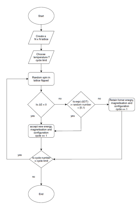
Implement a single cycle of the above algorithm in the montecarlocycle(T) function. This function should return the energy of your lattice and the magnetisation at the end of the cycle. You may assume that the energy returned by your energy() function is in units of $k_B$! Complete the statistics() function. This should return the following quantities whenever it is called: $<E>,<E^2>,<M>,<M^2>$, and the number of Monte Carlo steps that have elapsed.

def montecarlostep(self, T):
    "Executes Monte Carlo in a Single Step, updates the self quantities"
    e_old = self.energy()
    random_i = np.random.choice(range(0, self.n_rows)) # choose a random row, column to flip
    random_j = np.random.choice(range(0, self.n_cols))
    self.lattice[random_i][random_j] =  -self.lattice[random_i][random_j] # random spin flipped
    if self.energy() > e_old:
        Del_E = self.energy() - e_old
        p = np.e ** (-Del_E / T) # Monte Carlo condition
        random_number = np.random.random() # choose a random number in the range [0,1) # choose a random number in the range [0,1)

        if random_number > p:
            self.lattice[random_i][random_j] =  -self.lattice[random_i][random_j] # Monte Carlo Perturbation

    self.E  += self.energy() # Values of energy and magnetisation added to the self.properties
    self.E2 += self.energy() ** 2
    self.M += self.magnetisation()
    self.M2 += self.magnetisation() ** 2
    self.n_cycles += 1

    return self.energy(), self.magnetisation()

def statistics(self):
    "Return average values for various properties"
    return [self.E/self.n_cycles, self.E2/self.n_cycles, self.M/self.n_cycles, self.M2/self.n_cycles]

Animation of Monte Carlo Algorithim

Task 3

NOTE, ALL VALUES OF TEMPERATURE IN THE WORK ARE REPORTED IN UNITS OF $J{k}_B^{-1}$ NOT KELVINǃ

Animation of code is done in https://github.com/PanoptoSalad/Monte_Carlo_Ising_lattice/ILanim.py

If $T<T_C$, do you expect a spontaneous magnetisation (i.e. do you expect $⟨M⟩\ne 0$)? When the state of the simulation appears to stop changing (when you have reached an equilibrium state), use the controls to export the output to PNG and attach this to your report. You should also include the output from your statistics() function.

$T_C$ refers to the Curie temperature or critical temperature during phase transition. $⟨M⟩$ is the average spin state of the configuration. $⟨M⟩$ is an order parameter that is 0 beyond the critical point, but $\pm 1$ below it.

Plots of average energy and magentisation with cycle number for Units of temperature: (a) T = 0.1 (b) T = 1 (c) T = 2 (d) T = 3

$\mathrm{\Delta }F=\mathrm{\Delta }U-T\mathrm{\Delta }S$

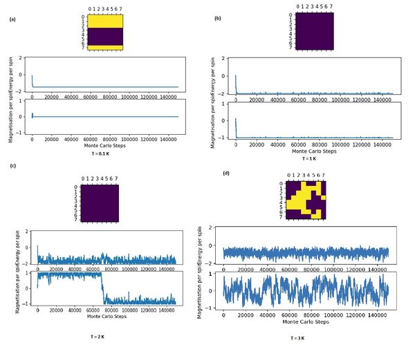
In this simulation, a canonical NVT ensemble is used since the lattice volume, the number of particles and temperature in the Monte Carlo simulation are fixed. The Helmholtz free energy $F$ is used because the simulation is done at constant volume.

Above Critical Temperature

For T = 3 : above critical temperature, the statistic() function prints:

[-112.27037777777778, 13021.761528888888, -12.429988148148148, 3238.0332325925924]

$⟨M⟩=-0.871$,

Above the curie Temperature, at T = 3 . a material loses its permanent magnetic properties because higher temperatures causes the entropic effects $\mathrm{\Delta }S$ to become more significant, making configurations with unaligned spin distributions more probable and demagnetisation spontaneous. $⟨M⟩=0$ The magnetisation is no longer at +1 or -1 as seen at lower temperatures, but fluctuates around 0. This is also illustrated by the local clumps of magnetic domains that spring up from a breakdown of order at higher temperatures. These oppositedly aligned domains cancel each other out on average.

At Critical Temperature

At the critical temperature of 2.27 K, fractals patterns begin to emerge and are spinodal decomposition like. This effect is most present at larger lattice sizes. Smaller lattice sizes fail to capture this effect at this temperature because of finite size effects that distort the critical temperature (further elaboration later) and also due to the 'zoomed-in' nature of the lattice that makes the patterns hard to identify.

Plot of 64 x 64 lattice at critical temperature

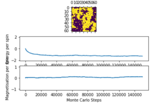
Below Critical Temperature

For T = 2: below critical temperature, the statistic() function prints:

[-116.72018346666667, 13833.826653866667, -11.709477333333334, 3354.4296874666666]

Note that the $⟨M⟩=-0.183$ due to spin flipping from the Monte carto algorithm identifying another energetically stable state of opposite spin.

For T = 1: below critical temperature, the statistic() function prints:

[-120.33467282051282, 14670.371798974358, 55.758445860189106,  3233.2315876923076]

$⟨M⟩=-0.871$, since the simulate equilibrates around spins +1 or -1 lowest energy state. The deviation from -1 is due to the inclusion of simulation properties prior to equilibration.

Below the curie temperature, the stability from exchange energy J of aligned spin states results in a configuration where the majority of spin states point in parallel, so $⟨M⟩\ne 0$. Entropic effects do not dominate, and the thermodynamic instability from the increase in microstates from flipping a spin is outweighed by the much greater fall in stability from loss of exchange energies at lower temperatures. Spontaneous magnetisation can then occur. Note that the stochastic perturbation from the Monte Carlo algorithm allows the simulation to cross unstable configurations and 'flip' spins, identifying 2 global minima in the process at T = 2.

Metastable states far below Critical Temperature

For T = 0.1: Metastable state, the statistic() function prints:

[-119.73041777777777 , 14535.222542222222, -6.757474444444444, 3162.881637777778]

Note that the $⟨M⟩=-0.105$ due to metastable state formation.

Note that metastable states (local minima) with 2 regions of oppositely aligned spins can possibly exist, making $⟨M⟩\approx 0$ a possibility at very low temperatures like 0.1 K. These oppositely spin aligned magnetic domains are next to each other and share an edge. At very low temperatures, the likelihood of a higher energy spin configuration being accepted by the algorithm is low. Thus, the system rapidly finds a local minimum and gets trapped there. This prevents the simulation from overcoming any energy barriers since the Monte Carlo perturbation is so tiny. This causes the configuration to be potentially stuck in metastable states since attempts to leave the local minima well involve temporarily passing through higher energy configurations which will be rejected by the algorithm.

Accelerating the code

Task 1

Use the script ILtimetrial.py: https://github.com/PanoptoSalad/Monte_Carlo_Ising_lattice/blob/main/ILtimetrial.py to record how long your current version of IsingLattice.py: https://github.com/PanoptoSalad/Monte_Carlo_Ising_lattice/blob/main/IsingLattice.py takes to perform 2000 Monte Carlo steps. This will vary, depending on what else the computer happens to be doing, so perform repeats and report the error in your average!

Using the unoptimised code:

Trial	Time Taken
1	8.1367264
2	8.740262900000001
3	8.740708299999998
4	9.101113300000002
5	8.341777700000002
6	8.1021662
7	7.997737199999996
8	8.645950400000004
9	8.720095999999998
10	8.850238300000001

The mean of time taken: 8.538 s The standard deviation of time taken: 0.369 s Hence:

$$\begin{gathered} time \\ taken=8.5\pm 0.4 \\ s \end{gathered}$$

Task 2

Look at the documentation for the NumPy sum function. You should be able to modify your magnetisation() function so that it uses this to evaluate M. The energy is a little trickier. Familiarise yourself with the NumPy roll and multiply functions, and use these to replace your energy double loop (you will need to call roll and multiply twice!).

def energy(self):
    L = np.sum( # Find energy of interactions with left neighbour
        np.multiply(np.roll(self.lattice, 1, 1), self.lattice))  
    R = np.sum(  # Find energy of interactions with right neighbour
        np.multiply(np.roll(self.lattice, 1, 0), self.lattice)) 
    return - L - R  # add the energies together

Task 3

Use the script ILtimetrial.py to record how long your new version of IsingLattice.py takes to perform 2000 Monte Carlo steps. This will vary, depending on what else the computer happens to be doing, so perform repeats and report the error in your average!

Using the optimised code:

Trial	Time Taken
1	0.38844220000009955
2	0.36627260000000206
3	0.401361100000031
4	0.39879019999989396
5	0.3895021999999244
6	0.39292550000004667
7	0.38721880000002784
8	0.3867660999999316
9	0.4128966999999193
10	0.39296969999986686

The mean of time taken: 0.391 s The standard deviation of time taken: 0.0120 s Hence:

$$\begin{gathered} time \\ taken=0.39\pm 0.01 \\ s \end{gathered}$$

This represents a 20 times improvement in the time taken for calculations. The substitution of python operations with that of numpy has sped up the calculations drastically. This is because of the way numpy stores its information in an array manner, and also because it is a library written in C++ code.

The effect of temperature

Correcting the Averaging Code

Task 1

A. The script ILfinalframe.py runs for a given number of cycles at a given temperature, then plots a depiction of the final lattice state as well as graphs of the energy and magnetisation as a function of cycle number. This is much quicker than animating every frame! Experiment with different temperatures and lattice sizes. How many cycles are typically needed for the system to go from its random starting position to the equilibrium state?

Equilibration and Lattice Size

Plots of energy and magentisation with step number for the various number of particles. Equilibration occurred more slowly for larger configurations

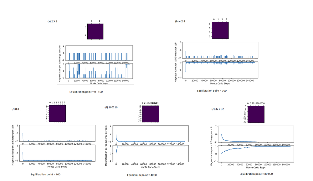
Equilibration time increased significantly with grid size. This is because more spins are present, with only one spin being flipped at a time, more steps are needed to ‘flip’ the randomly distributed spins from one state to the other since the equilibrium state involves all spins being in the one configuration. To make matters worse, since the choice of which lattice site to 'flip' is completely random, sites which are 'obviously' unstable to the human (like a singular up spin surrounded by down spin) might be missed by the simulation altogetherǃ The Monte Carlo algorithm is like throwing darts randomly at a board with a blindfold on, so the larger the board, the harder it is to hit the sweet spot to flip the right spin.

For systems of larger grid sizes, flipping two or more spins simultaneously might be an attractive strategy to cut equilibration time (as shown in extension).

This might not work for smaller size systems that suffer from finite-size effects since the two spins flipped will experience high correlation due to their close proximity from periodic boundary conditions.

Equilibration and Temperature

Plots of energy and magentisation with step number for various temperatures of simulations. Equilibration occurred faster for low temperatures, but equilibration time plateaus off beyond a certain temperature

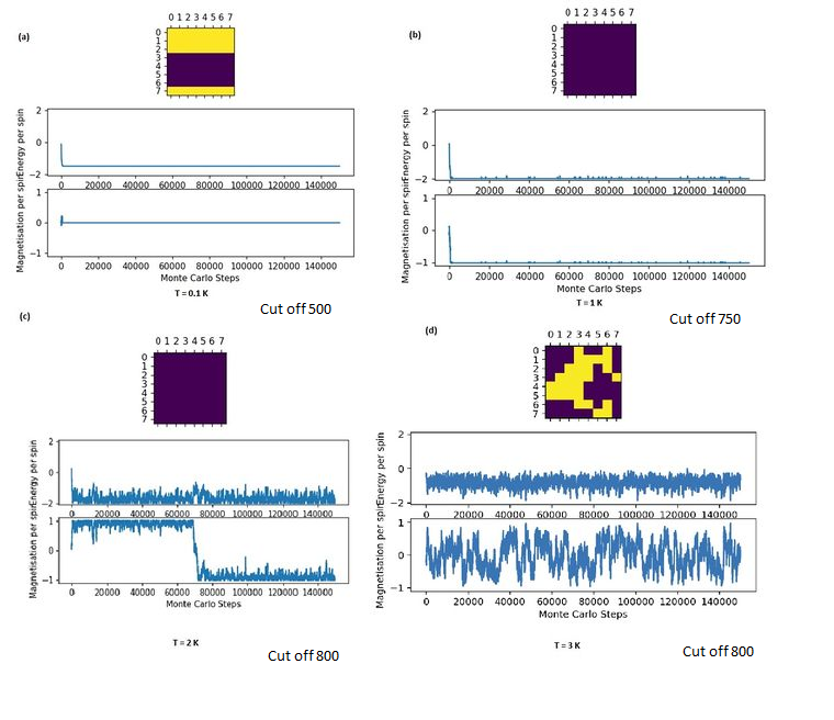
The system starts with an unoptimised random distribution of spins. When the temperature is lowered, the probability that a Boltzmann perturbation generates a higher energy state decreases, and the simulation is highly driven to rapidly find the most stable state, which is equilibrium when the magnetic spins are aligned. When the lattice size is kept constant, the system reaches equilibrium within a shorter number of cycles at lower temperatures than at higher temperatures. Beyond the critical temperature, however, the equilibrium has shifted to a lattice where long-range order has broken down and short-range local magnetic domains dominated. This is attained more easily from the initial random distribution since less order is present in the equilibrium state. This contrasts with the greater effort required to flip every spin to align in one direction at lower temperatures. At temperatures higher than the critical temperature, the equilibration time should stagnate or even decrease as the equilibrium position has shifted to a disorderly state that is easier to attain.

B. Modify your statistics() and montecarlostep() functions so that the first N cycles of the simulation are ignored when calculating the averages. You should state in your report what period you chose to ignore, and include graphs from ILfinalframe.py to illustrate your motivation in choosing this figure.

The approach towards implementing a cut-off point was to store the energy and magnetisation states per cycle in self.E_list and self.M_list. This has several advantages. The trajectory of the simulation of every cycle is preserved. These 2 lists can be converted into numpy.arrays() and their means can be obtained using numpy.mean() and standard deviations obtained using numpy.std(). The number of cycles can also be kept track of using len() to observe the length of the lists. There is no need for an 'if' condition to determine when to start storing the magnetisation and energy information. Instead, list or array slicing of using a cut-off point 'C_Off' can be used. This also bypasses the need to keep track of E2, M2, and number of cycles. The greater use of numpy to calculate means and standard deviations also make statistics calculations faster.

The main downside of such an approach is that the memory used for the calculations would be immense due to keeping track of the energy and magnetisation in a list for every step. For cycles involving millions of steps, the list will contain a million values that consume excess memory.

class IsingLattice:

    E_list = [] # List used instead of E, E2, M, M2
    M_list = []

    def montecarlostep(self, T):
        "Executes Monte Carlo in a Single Step, updates the self quantities"
        e_old = self.energy()
        random_i = np.random.choice(range(0, self.n_rows)) # choose a random row, column to flip
        random_j = np.random.choice(range(0, self.n_cols))
        self.lattice[random_i][random_j] *=  -1 # random spin flipped
        e_new = self.energy()
        if e_new > e_old:
            Del_E = e_new - e_old
            p = np.e ** (-Del_E / T) # Monte Carlo condition
            random_number = np.random.random() # choose a random number in the range [0,1)

            if random_number > p:
                self.lattice[random_i][random_j] =  -self.lattice[random_i][random_j]

        self.E_list.append(self.energy())
        self.M_list.append(self.magnetisation())

This new statistics() function is called statistics_capacity(self, C_Off) and takes in an argument regarding the cut-off point. This provides flexibility in choosing the cut-off for different equilibration times of different number of spins.

    def statistics_capacity(self, C_Off):
        "Return average values for various properties after a certain cutoff"
        return [np.mean(self.E_list[C_Off:]),
                np.std(self.E_list[C_Off:]) ,
                np.mean(self.M_list[C_Off:]),
                np.std(self.M_list[C_Off:]),
                np.mean(np.array(self.E_list[C_Off:])**2),
                np.mean(np.array(self.M_list[C_Off:])**2)
                ]

Running over a range of temperatures

Task 2

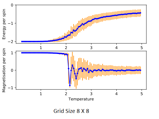
Use ILtemperaturerange.py from https://github.com/PanoptoSalad/Monte_Carlo_Ising_lattice/blob/main/ILtemperaturerange.py to plot the average energy and magnetisation for each temperature, with error bars, for an $8\times 8$ lattice. Use your intuition and results from the script ILfinalframe.py to estimate how many cycles each simulation should be. The temperature range of of 0.25 to 5.0 is sufficient. Use as many temperature points as you feel necessary to illustrate the trend, but do not use a temperature spacing larger than 0.5. The NumPy function savetxt() stores your array of output data on disk — you will need it later. Save the file as 8x8.dat so that you know which lattice size it came from.

Judging from the earlier section, the equilibrium was attained within 100,000 steps for all the various grid sizes and temperatures tested. It would make sense to use that as the standard total number of cycles used. Due to time constraints, larger cycles were not used. In hindsight.

Plots of Magnetisation, energy with temperature for 8X8 particles

The effect of system size

Task 1

A. Repeat the final task of the previous section for the following lattice sizes: 2x2, 4x4, 8x8, 16x16, 32x32. Make sure that you name each datafile that your produce after the corresponding lattice size! Write a Python script to make a plot showing the energy per spin versus temperature for each of your lattice sizes. Hint: the NumPy loadtxt function is the reverse of the savetxt function, and can be used to read your previously saved files into the script. Repeat this for the magnetisation. As before, use the plot controls to save your a PNG image of your plot and attach this to the report.

Code for ̈8 x 8 lattice Calculations to generate a .dat file

from IsingLattice import *

n_rows = 8
n_cols = 8
il = IsingLattice(n_rows, n_cols)
il.lattice = np.ones((n_rows, n_cols))
spins = n_rows*n_cols 
runtime = 100000 # set cycle number
times = range(runtime)
temps = np.arange(0.25, 5.0, 0.05) # Control the temperature range

energies = [] # Initialise empty lists to store data
magnetisations = []
energysq = []
magnetisationsq = []

for t in temps:    
    for i in times: # 2 for loops to run data over various temperature and various cycles
        il.montecarlostep(t)
        
    aveE, stdE, aveM, stdM, e2, m2 = il.statistics_capacity(2000) # 2000 arguments represents cut-off point for equilibrium
    energies.append(aveE)
    energysq.append(stdE)
    magnetisations.append(aveM)
    magnetisationsq.append(stdM)
    
    #reset the IL object for the next cycle
    il.n_cycles = 0
    il.E_list = []
    il.M_list  = []

final_data = np.column_stack((temps, energies, energysq, magnetisations, magnetisationsq))
np.savetxt("8x8.dat", final_data)

Code for reading a .dat file

from matplotlib import pylab as pl
import numpy as np

spins = 64

tempsls, energiesls, energysqls, magnetisationsls, magnetisationsqls = [],[],[],[],[] # initialise empty lists
for lines in np.loadtxt("8x8.dat"): # reads data off .dat file 
    temps, energies, energysq, magnetisations, magnetisationsq = lines # appends data to empty lists earlier
    tempsls.append(temps)
    energiesls.append(energies)
    energysqls.append(energysq)
    magnetisationsls.append(magnetisations)
    magnetisationsqls.append(magnetisationsq)

fig = pl.figure(figsize='10')

enerax = fig.add_subplot(2,1,1) # details of the 2 subplots provided
enerax.set_ylabel("Energy per spin")
enerax.set_xlabel("Temperature")
enerax.set_ylim([-2.1, 0])

magax = fig.add_subplot(2,1,2)
magax.set_ylabel("Magnetisation per spin")
magax.set_xlabel("Temperature")
magax.set_ylim([-1.1, 1.1])

enerax.plot(temps, np.array(energies)/spins,linestyle='-',marker='.',c='b')
enerax.errorbar(temps, np.array(energies)/spins,yerr=np.array(energysq)/spins,c='darkorange',linestyle='',markersize=1)

magax.plot(temps, np.array(magnetisations)/spins,linestyle='-',marker='.',c='b')
magax.errorbar(temps, np.array(magnetisations)/spins,yerr=np.array(magnetisationsq)/spins,c='darkorange',linestyle='',markersize=1)

pl.savefig('8x8.svg',bbox_inches='tight') # save an image
pl.tight_layout()
pl.show()

Plots of Magnetisation, energy with temperature for various number of particles in simulations.

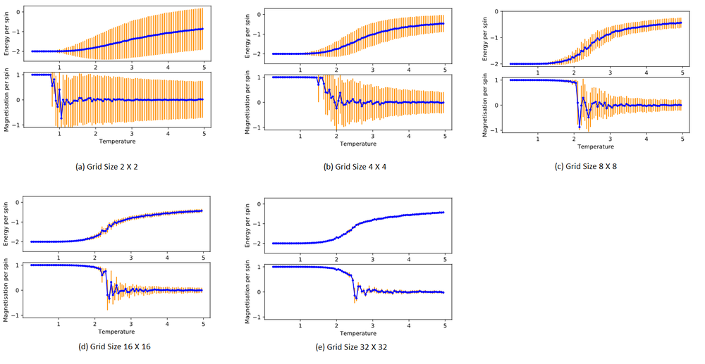
B. How big a lattice do you think is big enough to capture the long-range fluctuations?

Judging from the standard deviations from the plotted points, the large 16 x 16 and 32 x 32 lattices suffer the least from fluctuations in the cycles.

The bigger the lattice, the larger the sample size involved in an ensemble. The standard deviation is smaller when more samples are considered, as thermal fluctuations tend to cancel out. The impact of a high energy spin-flip at a Monte Carlo perturbation step affects the total energy or magnetisation less when there are more spins involved. The 2 X 2 system experiences high standard deviation when even just 1 spin-flip occurs from the perturbation. This creates massive fluctuations and high standard deviations.

Another major problem introduced by small lattices is the finite-size effects mentioned earlier. These problems result from the periodic boundary conditions of finite-sized lattices. Even though each spin of a lattice site only interacts directly with its edge-sharing neighbours, in reality, the spin of a lattice site influence its neighbours, and the neighbours' spin affects their neighbours and so on and so forth. The correlation length ξ and correlation function Γ measures this.

ː$\mathrm{\Gamma }({\hat{r}}_i,{\hat{r}}_j)=⟨s_i{s}_j⟩-⟨s{⟩}^2$

Where $widehat{r}_i,{\hat{r}}_j$ are the position vectors of the spins of interest, and $s_i$ and $s_j$are their spins.

$⟨S⟩$ is the average spin per lattice site, or the net lattice magnetisation per spin. Above the critical temperature:

ː$\mathrm{\Gamma }\sim {\mathrm{r}}^{-\tau }\exp (-r/\xi )$

Γ is a function of distance. τ is some number. Away from the critical point, the spins are uncorrelated, as their influence on each other becomes increasingly irrelevant. At distances close to each other, the correlation between spins is stronger. The larger the correlation length ξ, the stronger the correlation between spins.

ː$\xi \sim {|T-T_C|}^{-v}$

Γ is also a function of temperature. At high temperatures T, Γ decreases to 0, since the spins are randomly distributed. When the temperatures decrease to the critical temperature T_C and the correlation length ξ diverges, increasing to ∞ due to an establishment of magnetic order. When the correlation length is small relative to the lattice length, finite-size correction effects are not dominant. However, if the correlation length is comparable to the lattice length, the periodic boundary conditions cause a lattice site spin to interact and influence its own behaviour. For instance, in a 2 x 2 lattice, if the top left site is spin up, it might end up encouraging itself to remain up due to correlation effects. In contrast, in a 32 X 32 system, the top left spin is 32 lattice site spacings away from itself (due to PBC) and experience much weaker long-range correlation effects. At critical temperatures, Γ→∞, so finite-size effects distort behaviour and cause deviations even for large lattice sizes. These fluctuations can be partially compensated for by using larger lattices like 16 x 16 or 32 x32. Their effects are most dominant for smaller lattices like 2 x 2, 4 x 4 and 8 x 8.

Determining the heat capacity

The heat capacity is a metric that aids the identification of the critical point.

Task 1

By definition,

$C=\frac{\partial ⟨E⟩}{\partial T}$

From this, show that

$C=\frac{\mathrm{V}\mathrm{a}\mathrm{r}[E]}{k_B{T}^2}$

Proof:

$⟨E{⟩}_T=\frac{1}{Z}\sum _{\alpha }E(\alpha )\exp \{-\frac{E(\alpha )}{k_{B}T}\}$

${⟨E^2⟩}_T=\frac{1}{Z}\sum _{\alpha }{E}^2(\alpha )\exp \{-\frac{E(\alpha )}{k_{B}T}\}$

$Z=\sum _{\alpha }\exp \{-\frac{E(\alpha )}{k_{B}T}\}$

The above equations are definitions for the expectation values of the energy E and E2 respectively. Z is the partition function.

$\frac{\partial ⟨E{⟩}_T}{\partial T}=\frac{\partial }{\partial T}{[\sum _a\exp \{-\frac{E(\alpha )}{k_{B}T}\}]}^{-1}+\frac{\partial }{\partial T}\frac{1}{Z}\sum _{\alpha }E(\alpha )\exp \{-\frac{E(\alpha )}{k_{B}T}\}$

Using product rule, the above derivative can be split into the two following components

Component 1

$\begin{array}{rl}\frac{\partial }{\partial T}{[\sum _a\exp \{-\frac{E(\alpha )}{k_{B}T}\}]}^{-1}& =-{[\sum _{\alpha }\exp \{-\frac{E(\alpha )}{k_{B}T}\}]}^{-2}\sum _{\alpha }\frac{E(\alpha )}{k_B{T}^2}\exp \{-\frac{E(\alpha )}{k_{B}T}\}\\ & =-Z^{-2}\sum _{\alpha }\frac{E(\alpha )}{k_B{T}^2}\exp \{-\frac{E(\alpha )}{k_{B}T}\}\end{array}$

Component 2

$\frac{\partial }{\partial T}\sum _{\alpha }E(\alpha )\exp \{-\frac{E(\alpha )}{k_{B}T}\}=\sum _{\alpha }\frac{E(\alpha )}{k_B{T}^2}E(\alpha )\exp \{-\frac{E(\alpha )}{k_{B}T}\}$

Combining the two equations, one can getː

$\begin{array}{rl}\frac{\partial ⟨E{⟩}_T}{\partial T}& =-Z^{-2}{[\sum _{\alpha }\frac{E(\alpha )}{k_B{T}^2}\exp \{-\frac{E(\alpha )}{k_{B}T}\}]}^2+\frac{1}{z}\sum _{\alpha }\frac{E(\alpha )}{k_B{T}^2}E(\alpha )\exp \{-\frac{E(\alpha )}{k_{B}T}\}\\ & =-\frac{1}{Z^2{k}_B{T}^2}{[\sum _{\alpha }E(\alpha )\exp \{-\frac{E(\alpha )}{k_{B}T}\}]}^2+\frac{1}{Z{k}_B{T}^2}\sum _{\alpha }{E}^2(\alpha )\exp \{-\frac{E(\alpha )}{k_{B}T}\}\\ & =-\frac{⟨E{⟩}_T^2}{k_B{T}^2}+\frac{{⟨E^2⟩}_T}{k_B{T}^2}\end{array}$

Sample variance S (square of standard deviation σ) is given byː

$\mathrm{V}\mathrm{a}\mathrm{r}[E]={\sigma }^2=\frac{\sum _a{E}_a^2-\frac{{\left(\sum _a{E}_a\right)}^2}{n}}{n}={⟨E^2⟩}_T-⟨E{⟩}_T^2$

For large values of n,

$\mathrm{V}\mathrm{a}\mathrm{r}[E]={⟨E^2⟩}_T-⟨E{⟩}_T^2$

Substituting this into the previous derivative,

$C=\frac{\partial ⟨E{⟩}_T}{\partial T}=\frac{{\sigma }^2}{k_B{T}^2}$

Task 2

Write a Python script to make a plot showing the heat capacity versus temperature for each of your lattice sizes from the previous section. You may need to do some research to recall the connection between the variance of a variable, $\mathrm{V}\mathrm{a}\mathrm{r}[X]$, the mean of its square $⟨X^2⟩$, and its squared mean ${⟨X⟩}^2$. You may find that the data around the peak is very noisy — this is normal and is a result of being in the critical region. As before, use the plot controls to save your a PNG image of your plot and attach this to the report.

Code

from matplotlib import pylab as pl
import numpy as np

tempsls32, energiesls32, energysqls32, magnetisationsls32, magnetisationsqls32 = [],[],[],[],[] # intialise empty list
for lines in np.loadtxt("32x32.dat"):
    temps, energies, energysq, magnetisations, magnetisationsq = lines
    tempsls32.append(temps)
    energiesls32.append(energies)
    energysqls32.append(energysq)
    magnetisationsls32.append(magnetisations)
    magnetisationsqls32.append(magnetisationsq)
    
tempsls32 = np.array(tempsls32)
energysqls32 = np.array(energysqls32)
capacity32 = energysqls32**2 / tempsls32**2

fig = plt.figure(figsize=(5,5))
cap1 = fig.add_subplot(1,1,1)
cap1.plot(tempsls32,capacity32/32**2, c = 'blue') # find the specific heat capacity per spin
cap1.set_ylabel(r"Specfic Heat capacity / $k_{b}\ JK^{-1}$ ") 
cap1.set_xlabel("Temperature / K")
#pl.savefig('hc3232.svg',bbox_inches='tight')

Plots of Magnetisation, energy with temperature for various number of particles in simulations.

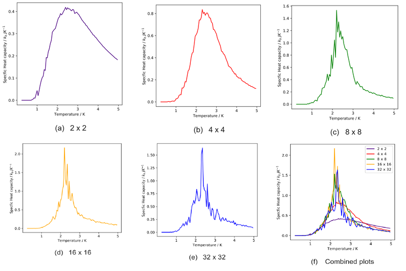
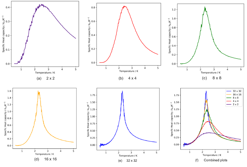
As mentioned earlier, an asymptotic singularity is expected during the phase transition. However, the finite-size effects result in maxima instead of the plots. The critical temperature would also be thrown off from the analytical value of critical temperature. The only way to achieve singularity is to use an infinitely large lattice, which is not computationally feasible and will take forever to equilibrate. The solution to this conundrum will be shown later.

Locating the Curie temperature

Task 1

A C++ program has been used to run some much longer simulations than would be possible on the college computers in Python. Plot the C++ data against your data. For one lattice size, save a PNG of this comparison and add it to your report — add a legend to the graph to label which is which.

Plots of Magnetisation, energy with temperature for various number of particles in simulations.

Polynomial fitting

Task 2

write a script to read the data from a particular file, and plot C vs T, as well as a fitted polynomial. Try changing the degree of the polynomial to improve the fit — in general, it might be difficult to get a good fit! Attach a PNG of an example fit in your report.

Code for reading .dat file and plotting graph

from matplotlib import pylab as pl
import numpy as np

# Reading file
tempsls16c, energiesls16c, energysqls16c, magnetisationsls16c, magnetisationsqls16c = [],[],[],[],[] # intialise empty list
for lines in np.loadtxt("16x16.dat"): # loop through file
    temps, energies, energysq, magnetisations, magnetisationsq = lines
    tempsls16c.append(temps)
    energiesls16c.append(energies)
    energysqls16c.append(energysq)
    magnetisationsls16c.append(magnetisations)
    magnetisationsqls16c.append(magnetisationsq) # Store data into the empty lists made earlier

tempsls16c = np.array(tempsls16c) # converting lists to numpy arrays for easier handling
energystd16c = np.array(energysqls16c)-np.array(energiesls16c)**2
capacity16c = energystd16c / (tempsls16c**2) # Deriving heat capacity from variance of energy and temperature

# Plotting graph
fig = plt.figure(figsize=(5,5))
cap1 = fig.add_subplot(1,1,1)
cap1.plot(tempsls16c,capacity16c/16**2, c = 'blue') # find the specific heat capacity per spin
cap1.set_ylabel(r"Specfic Heat capacity / $k_{b}\ JK^{-1}$ ") 
cap1.set_xlabel("Temperature / K")
pl.savefig('hc1616.svg',bbox_inches='tight')

Code for fitting and plotting data

c16c = capacity16/16**2 # retrive the heat capacity from previously

fit3 = np.polyfit(tempsls16c, c16c, 3)  # polynomial fit of data with polynomials of various orders
fit4 = np.polyfit(tempsls16c, c16c, 4)
fit5 = np.polyfit(tempsls16c, c16c, 5)
fit6 = np.polyfit(tempsls16c, c16c, 6)

fig = plt.figure(figsize=(5,5))
cap1 = fig.add_subplot(1,1,1)
cap1.plot(tempsls16c,c16c, c = 'darkorange',marker='.',linestyle='') # plotting actual data

x3_16c = np.linspace(0.5,5,1000) # generating temperature data to evaluate fit effectiveness
    
y3_16c = np.polyval(fit3, x3_16c) # generating heat capacity data to evaluate fit effectiveness
y4_16c = np.polyval(fit4, x3_16c)
y5_16c = np.polyval(fit5, x3_16c)
y6_16c = np.polyval(fit6, x3_16c)

cap1.plot(x3_16c,y3_16c,linestyle='--',c='blue',label='3rd Order') # plotting various fits
cap1.plot(x3_16c,y4_16c,linestyle='--',c='green',label='4th Order')
cap1.plot(x3_16c,y5_16c,linestyle='--',c='red',label='5th Order')
cap1.plot(x3_16c,y6_16c,linestyle='--',c='indigo',label='6th Order')

cap1.set_ylabel(r"Specfic Heat capacity / $k_{b}\ JK^{-1}$ ")
cap1.set_xlabel("Temperature / K")
cap1.legend()
plt.savefig('fitting.svg',bbox_inches='tight')

Plot of heat capacity against temperature. Various fits of different polynomial orders are used to attempt to fit the data.

Despite increasing the order of the polynomial fit, the plot did not appear to be fit the curves better. Using a polynomial fit does not seem to yield convergence.

Task 3

A. Find the temperature at which the maximum in C occurs for each datafile that you were given.

Plots of heat capacity and temperature at various grid sizes. A 6th order polynomial fit was used about the maxima regions

The lattice lengths and critical temperatures from the fits are given below. Finite-size effects and correlation lengths cause the critical temperature detected to be different for different lattice sizes. It also causes maxima to be obtained instead of the first-order transition anticipated.

Lattice length           Critical Temperature
2.000000000000000000e+00 2.504804804804804608e+00
4.000000000000000000e+00 2.452902902902903026e+00
8.000000000000000000e+00 2.338988988988988993e+00
1.600000000000000000e+01 2.307307307307307376e+00
3.200000000000000000e+01 2.294344344344344311e+00

Due to finite size effects, the critical temperature is related to the system size byː

ː$T_{C,L}=\frac{A}{L}+T_{C,\mathrm{\infty }}$

This equation is a good approximation to predict the critical temperature

B. Make a plot that uses the scaling relation given above to determine $T_{C,\mathrm{\infty }}$. By doing a little research online, you should be able to find the theoretical exact Curie temperature for the infinite 2D Ising lattice. How does your value compare to this? Are you surprised by how good/bad the agreement is? Attach a PNG of this final graph to your report, and discuss briefly what you think the major sources of error are in your estimate.

Plot of Curie Temperature against inverse of lattice length to show finite size effects

Values for the $T_{C,\mathrm{\infty }}$ obtainedː $T_{C,\mathrm{\infty }}=2.25\pm 0.04$ matches the literature value that states Onsager's analytical value of critical temperature asː

$k_B{T}_c/J=\frac{2}{\ln (1+\sqrt{2})}\approx 2.26918531421$

This is a difference of less than 1%. This is rather impressive. The main sources of error that could have affected these results are a lack of data points and repetition. The data for the c++ code provided largely follow the linear trend, but 16 x 16 lattice seems to deviate significantly from the trend and might have contributed significantly to the error. Also, another inaccuracy comes from only using 5 data points to obtain the linear fit. With more data, the fit could be better. The variance in heat capacity from the c++ code is also unknown since repeats are not performed. With more repeats of the same data points, the results will be more accurate and a weighted linear fit can be used as well. Another minor source of error might originate from the fitting of the function with the numpy polyfit function. Some statistical errors might also come from the noise in stochastic methods, or from variations during the sampling process.

Extensionsː Potts Model

Background

The Potts' model allows the spin to adopt a q number of configurations about a circle. In the Ising model, q = 2. The angles permitted are:

${\theta }_n=\frac{2\pi n}{q}$

In the continuous spin model q is allowed to go to ∞, the spins can adopt any spin direction θ, instead of just +1 or -1. This is reflected in the following code when each lattice site is assigned a random number between 0 to 2 π. This reflects the direction of the spin.

Code for Potts Model Part 1

import numpy as np

class IsingLattice:

    E_list = []
    M_list  = []

    def __init__(self, n_rows, n_cols):
        self.n_rows = n_rows
        self.n_cols = n_cols
        self.lattice = np.random.choice(np.arange(0,2*np.pi,0.001), size=(n_rows, n_cols)) # gives a lattice of random angles

Once this restriction on spin has been lifted, the Hamiltonian will differ. This is because the spin is a 2D vector with direction and magnitude. A dot product will have to be incorporated.

$H=-J\sum _{(i,j)}{\mathbf{s}}_i\cdot {\mathbf{s}}_j-\sum _j{\mathbf{h}}_j\cdot {\mathbf{s}}_j$

In the XY model, the magnitude of the spins is set to 1. In this section, the external field was treated to be zero. This simplifies the expression as energy is now a function of the cosine of the difference in angle between neighbouring sites.

$H=-J\sum _{(i,j)}\cos ({\theta }_{s_i}-{\theta }_{s_j})$

The magnetisation is now a vector sum and rather than a simple scalar addition.

    def energy(self):
        "Return energy by doing a dot product"
        L = np.cos(np.roll(self.lattice, 1, 1)- self.lattice) # energy is found by taking a cosine of the difference in angles in lattices
        R = np.cos(np.roll(self.lattice, 1, 0)- self.lattice)
        return np.sum(-L-R)

    def magnetisation(self):
        "Return the magnetisation magnitude of the current lattice configuration."
        x = np.sum(np.cos(self.lattice)) # the x and y components of the net magnetisation are found
        y = np.sum(np.sin(self.lattice))
        complex1 = complex(x,y)
        return [np.absolute(complex1),np.angle(complex1)] # magnetisation vector made to complex number

The Monte Carlo algorithm is also modified to pick a random number between 0 to 2π to perturb a current lattice site's spin by rather than just flipping a spin by -1

    def montecarlostep(self, T):
        "Executes Monte Carlo in a Single Step, updates the self quantities"
        e_old = self.energy()
        shape = np.copy(self.lattice)
        random_i = np.random.choice(range(0, self.n_rows)) # choose a random row, column to flip
        random_j = np.random.choice(range(0, self.n_cols))
        lattice_old = self.lattice[random_i][random_j]

        self.lattice[random_i][random_j] +=  np.random.random() * 2 * np.pi # random spin flipped by random amount
        if self.lattice[random_i][random_j] > 2 * np.pi: # periodic conditions, prevent angle from being too big
            self.lattice[random_i][random_j] -= 2 * np.pi
        e_new = self.energy()
        if e_new > e_old:
            Del_E = e_new - e_old
            p = np.e ** (-Del_E / T) # Monte Carlo condition
            random_number = np.random.random() # choose a random number in the range [0,1)

            if random_number > p:
                self.lattice[random_i][random_j] = lattice_old

        eng = self.energy()
        mag = self.magnetisation()
        return [eng,mag,shape] # outputs the energy, magnetisation vector, and lattice shape

Implementing Monte Carlo Steps

This script will read an input file containing information regarding the lattice size, temperature and number of cycles and produce 2 output files showing the simulation behaviour every cycle. The name of the file will be the same for output and inputs. Only the extension changes.

Input file: File:Input1.in Output data file: File:Input1.dat and File:Input1.traj

# Reads an input file, produces an output file with magnetism, energy as an .dat file. Also produces a trajectory file .traj illustrating the lattice site spins per cycle

from IsingLattice_magnet import *

filename = input('Please put in file name: ')

f=open('{}'.format(filename), "r") # reads the input file
data = []
for i in f.readlines():
    data.append(i.split()[-1]) # reads the last string (seperated by ' ') of each line
f.close()

N = int(data[0]) # Lattice length
T = float(data[1]) # Temperature 
cycles = int(data[2]) # Number of cycles implemented
filename = filename.split('.')[0] # Output file name

il = IsingLattice(N,N) # create a 2D lattice of the class Isinglattice
spins = N*N

e_list = [] # energy of the 
mag_abs = [] # magnetism stored as a complex number, absolute value
mag_ang = [] # the angle of the complex number
l_list = [] # stores the lattice angles 

def animate(runs,temperature):
    ' Does a monte carlo step and appends various properties to list above '
    for _ in range(runs):
        energy, magnetisation,shape = il.montecarlostep(temperature) # uses output defined in IsingLattice_magnet.py
        e_list.append(energy)
        mag_abs.append(magnetisation[0])
        mag_ang.append(magnetisation[1])
        l_list.append(shape)        

animate(cycles,T) # Run the monte carlo simulation over a certain number of cycles

# From this point onwards code stores the data produced

final_data = np.column_stack((e_list,mag_abs,mag_ang))
np.savetxt("{}.dat".format(filename), final_data) # storing the net magnetisation, energy data
with open('{}.dat'.format(filename), 'a') as outfile:
	outfile.write('# {} {} {} '.format(N,T,cycles))

# Deals with storing the lattice site data at each cycle. 
# Lattice data has a shape of Number of cycles x number of rows x number of columns. 3D array.

data = np.array(l_list)

with open('{}.traj'.format(filename), 'w') as outfile:
    outfile.write('# Array shape: {0}\n'.format(data.shape)) # creates a header with information about data array
    
    for data_slice in data:
        np.savetxt(outfile, data_slice) # Stores the lattice data at each cycle
        outfile.write('# New cycle\n') # new cycle comment between each cycle

Animation

This script takes in a .traj file produced earlier and animates it as an mp4 file

from matplotlib import pylab as plt
from matplotlib import animation
import numpy as np
import re

filename = input('Please put in trajectory file name (.traj): ')

first_line1 = open(filename,'r')
first_line = first_line1.readlines()[0]
first_line1.close()
cycles,rows,cols =  re.findall(r"[\w']+", first_line)[2:]
cycles = int(cycles)
rows = int(rows)
cols = int(cols)

new_data = np.loadtxt(filename) 

# this produces a 2D array from original 3D array
# We can restore 3D array if we know the shape as stored in the comment earlier

l_list = new_data.reshape(cycles, rows, cols)

fig = plt.figure()
ax = plt.subplot(111)

ax.xaxis.set_ticks([])
ax.yaxis.set_ticks([])

line = ax.matshow(l_list[0], cmap='hsv', vmin=0, vmax=2*np.pi)

def update(i):
    line.set_data(l_list[i])
    return line,

anim = animation.FuncAnimation(fig, update,interval=0,save_count=cycles, blit=True)
plt.colorbar(line,label='Spin direction from '+ r'$0 - 2\pi$')

anim.save('{}_latticetraj.mp4'.format(filename.split('.')[0]), fps=30)

Results

https://www.youtube.com/watch?v=puknlkcMdq4
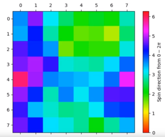
Video Illustrating the first 1000 steps of a 8 x 8 XY model lattice at 0.1 temperature units

For an 8 x 8, equilibration is achieved when the colours of the lattice sites cluster around a particular region. This is achieved at temperatures below the critical point.

When the temperature is raised above the critical point at 2.5 temperature units, the equilibrium configuration favours a random distribution instead.

https://www.youtube.com/watch?v=nS7wBZSP9d4&feature=youtu.be
Video Illustrating the first 10000 steps of a 8 x 8 XY model lattice at 2.5 temperature units

https://www.youtube.com/watch?v=F7eG4cVyPVI&feature=youtu.be
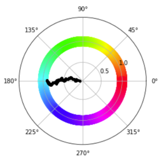
Video Illustrating the magnetisation trajectory of the first 10000 steps of a 8 x 8 XY model lattice at 0.1 temperature units

The magnetisation vector trajectory for the lattice spin can be visualised using a polar plot to show the magnitude and direction per spin. Initially, the net magnetisation magnitude is 0. It slowly increases with time to approach 1, showing that the spins are now all aligned. The starting net direction of the spin affects the final net direction of the spins.

The simulation was then run for 500,000 cycles for a 32 x 32 system, and the video of the animation is as shown:

https://www.youtube.com/watch?v=HDdifkqIMhM
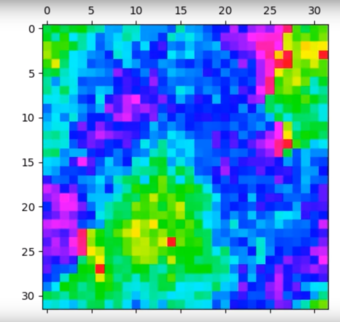
Video Illustrating the approximately 250,000 cycles of a 32 x 32 XY model lattice at 0.1 temperature units

Illustration of the evolution of the 32 x 32 XY model lattice at 0.1 temperature units simulation with cycle number 1 million

Extensions: Spinodal Decomposition

Illustration of the evolution of the 100 x 100 ising lattice at 2.26 temperature units over 10 million cycles

When letting the simulation run at the critical temperature, spinodal decomposition can be seen, due to the curved magnetic domains.

Illustration of the evolution of the 100 x 100 ising lattice at 2.26 temperature units over 1 million cycles

To speed up equilibration, 4 random lattice sites were chosen and flipped simultaneously using the modified code below.

    def montecarlostep(self, T):
        "Executes Monte Carlo in a Single Step, updates the self quantities"
        e_old = self.energy()
        lat_old = np.copy(self.lattice)
        random_i = np.random.choice(range(0, self.n_rows)) # choose a random row, column to flip
        random_j = np.random.choice(range(0, self.n_cols))
        random_j1 = np.random.choice(range(0, self.n_cols))
        random_i1 = np.random.choice(range(0, self.n_rows))
        random_j2 = np.random.choice(range(0, self.n_cols))
        random_i2 = np.random.choice(range(0, self.n_rows))
        random_j3 = np.random.choice(range(0, self.n_cols))
        random_i3 = np.random.choice(range(0, self.n_rows))

        self.lattice[random_i][random_j] *=  -1 # random spin flipped
        self.lattice[random_i1][random_j1] *=  -1 # random spin flipped
        self.lattice[random_i2][random_j2] *= -1  # random spin flipped
        self.lattice[random_i3][random_j3] *= -1  # random spin flipped

        e_new = self.energy()
        if e_new > e_old:
            Del_E = e_new - e_old
            p = np.e ** (-Del_E / T) # Monte Carlo condition
            random_number = np.random.random() # choose a random number in the range [0,1)

            if random_number > p:
                self.lattice = lat_old

        self.E_list.append(self.energy())
        self.M_list.append(self.magnetisation())

        return self.energy(), self.magnetisation()

Extension: External magnetic Field

An additional argument f can be used for external field

    def energy(self,F):
        L = np.sum( # Find energy of interactions with left neighbour
            np.multiply(np.roll(self.lattice, 1, 1), self.lattice))
        R = np.sum(  # Find energy of interactions with right neighbour
            np.multiply(np.roll(self.lattice, 1, 0), self.lattice))
	M = F * self.lattice
        return - L - R - M  # add the energies together

Bibliography

- ↑ E. Schneidman, M. J. Berry II, R. Segev and W. Bialek,Nature, 2006,440, 1007
- ↑ E. Ising, Z. Phys., 1925,31, 253–258.
- ↑ S. M. Bhattacharjee and A. Khare,Current science, 1995,69, 816–821
- ↑ J. M. Yeomans, Statistical mechanics of phase transitions, ClarendonPress, 1992
- ↑ K. Binder, D. Heermann, L. Roelofs, A. J. Mallinckrodt and S. McKay, Computers in Physics, 1993,7, 156–157.
- ↑ L. Knox, N. Christensen and C. Skordis,The Astrophysical JournalLetters, 2001,563, L95.
- ↑ R. Y. Rubinstein and D. P. Kroese, Simulation and the Monte Carlo method, John Wiley & Sons, 2016, vol. 10.
- ↑ S. Van Der Walt, S. C. Colbert, and G. Varoquaux, Computing in Science & Engineering, 2011,13, 22.
- ↑ J. M. Yeomans,Statistical mechanics of phase transitions, ClarendonPress, 1992.
- ↑ B. M. McCoy and T. T. Wu,The two-dimensional Ising model, CourierCorporation, 2014.