Rep:CMPY3 GE715

Ising Model

Ising model is built on the assumption that a lattice that can be of any dimensionality contains spins which can either be up (+1 or down (-1) and interactions can be studied using this model. The model is extremely simplified, since in real systems the spins can point in any direction, but the basic properties of magnetic systems, such as magnetisation, energy levels and Curie temperature, may be studied using this simplification.

The interaction energy in Ising model is defined as $E = - \frac{1}{2} J \sum_{i}^{N} \sum_{j \in n e i g h b o u r s (i)} s_{i} s_{j}$ . The energy will be the lowest possible when all the spins point in the same direction. In that case $s_{i} s_{j} = 1$ for all possible $i, j$ pairs. The number of pairs for each $i$ depends on the number of dimensions.

$P = 2 D$ , where $P$ represents the number of pairs and $D$ the number of dimensions. The lowest possible energy will thus be $E = - \frac{1}{2} J N P$ , where $N$ represents the total number of spins. Thus the lowest possible energy may also be simplified as $E = - D N J$ , as requested.

The multiplicity of this particular state is 2 (all spins up or all spins down), thus $Ω = 2$ , entropy of the system is $S = k_{b} l n Ω = 9.6 * 1 0^{- 24} J K^{- 1}$ .

Flip of a spin

If one of the spins flips, the energy increases. In the given case ( $D = 3, N = 1000$ ), the $E_{i} = - 3000 J$ , while the flip of one spin increases the energy by $12 J$ (6 pairs, $2 J$ per pair), so that $E_{f} = - 2988 J$ . Note that $J$ does not represent joules in this case.

Multiplicity has increased to $Ω = 2000$ , thus $S = 1.05 * 1 0^{- 22} J K^{- 1}$ .

$Δ S = 1.04 * 1 0^{- 22} J K^{- 1}$ .

This means that entropy has increased by more than 100 times.

Magnetisation in the sketch

The 1D system shown has the magnetisation of $M = 1$ . This is also true for the 2D system shown. For the model system with $N = 1000, D = 3$ the expected magnetisation at absolute zero would be $M = \pm 1000$ .

Code for magnetisation and energy

Python code was written to calculate the energy and magnetisation of a configuration and tested a few times. The test results are shown in figure 1 below.

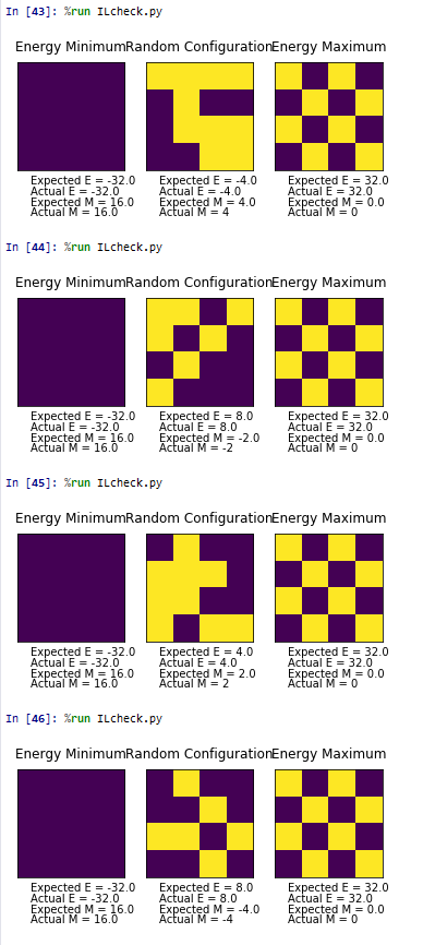Figure 1: Test results

Monte Carlo simulation

If no weighing is used, the calculation would be far too demanding even for current supercomputers, because 100 spins can take about $1.27 * 1 0^{30}$ arrangements, which means calculating the average for such system would take more than $1.3 * 1 0^{21} s$ , which is 40 trillion years, or about 3 times the age of the Universe, thus a better system must be used to do this quicker. One option is using Monte Carlo simulation, which mimics real transitions. It is essentially optimisation algorithm that is looking for stable state, but with a possibility of going into higher energy state should it have enough energy.

Below Curie temperature it is to be expected, that absolute value of magnetisation will be close to LxL, where L is the size of the lattice (works also in more than 2 dimensions).

The old code was accidentally deleted before it could be added to the report.

Accelerating the code

The code at the beginning was written using a loop for magnetisation and a double loop for energy. 2000 Monte Carlo steps needed was $M = 9.32 s \pm 0.10 s$ . After optimizing magnetisation only this has dropped to $M = 8.88 s \pm 0.04 s$ , while after optimizing both magnetisation and energy with using Numpy's sum, roll and multiply functions, the time was further reduced to $M = 0.0796 s \pm 0.018 s$ . It was later realised that only one roll in each direction is needed to produce the correct energy, so the final time for 2000 steps was successfully reduced to $M = 0.418 s \pm 0.005 s$ .

The whole of the code used is given below.

import numpy as np

class IsingLattice:

    E = 0.0
    E2 = 0.0
    M = 0.0
    M2 = 0.0
    energy_x=0
    energy2_x=0
    magnetisation_x=0
    magnetisation2_x=0

    n_cycles = 0

    def __init__(self, n_rows, n_cols):
        self.n_rows = n_rows
        self.n_cols = n_cols
        self.lattice = np.random.choice([-1,1], size=(n_rows, n_cols))

    def energy(self):
        a=np.roll(self.lattice,1,axis=0)
        a1=np.multiply(a,self.lattice)
        x1=np.sum(a1)
        c=np.roll(self.lattice,1,axis=1)
        c1=np.multiply(c,self.lattice)
        x2=np.sum(c1)
        x=x1+x2
        energy = -x
        return energy

    def magnetisation(self):
        "Return the total magnetisation of the current lattice configuration."
        return np.sum(self.lattice)

    def energy_flip(self,random_i,random_j):
        "Return the total energy of the current lattice after flip configuration."
        self.lattice[random_i][random_j]=-self.lattice[random_i][random_j]
        a=np.roll(self.lattice,1,axis=0)
        a1=np.multiply(a,self.lattice)
        x1=np.sum(a1)
        c=np.roll(self.lattice,1,axis=1)
        c1=np.multiply(c,self.lattice)
        x2=np.sum(c1)
        x=x1+x2
        energy = -x
        return energy

    def montecarlostep(self, T):
        # complete this function so that it performs a single Monte Carlo step
        energy = self.energy()
        #the following two lines will select the coordinates of the random spin for you
        random_i = np.random.choice(range(0, self.n_rows))
        random_j = np.random.choice(range(0, self.n_cols))
        #the following line will choose a random number in the range [0,1) for you
        random_number = np.random.random()
        self.lattice[random_i][random_j] = -self.lattice[random_i][random_j]
        energy2 = self.energy()
        dE = energy2 - energy

        if energy2<energy or random_number<=np.e**(-(energy2-energy)/T):
            yyy=True
        else:
            self.lattice[random_i][random_j] = -self.lattice[random_i][random_j]
			
        self.n_cycles+=1

        self.E += self.energy()
        self.E2 += self.energy()**2
        self.M += self.magnetisation()
        self.M2 += self.magnetisation()**2
        return self.energy(), self.magnetisation()

    def statistics(self):
        # complete this function so that it calculates the correct values for the averages of E, E*E (E2), M, M*M (M2), and returns them
        avE = self.E / self.n_cycles
        avE2 = self.E2 / self.n_cycles
        avM = self.M / self.n_cycles
        avM2 = self.M / self.n_cycles
        return avE, avE2, avM, avM2, self.n_cycles

Temperature effects

Correction of averaging code

A few experiments were performed at different temperatures using ILfinalframe.py, to see how long it usually takes for the system to equilibrate. At low temperatures it usually happened before 1000 steps were performed, thus 1000 Monte Carlo steps was decided to be appropriate cut-off period for calculation of average values of magnetisation and energy. The figures 2-4, showing the experiments performed are shown in the gallery below.

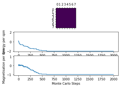Figure 2: Test result @ 0.5 K
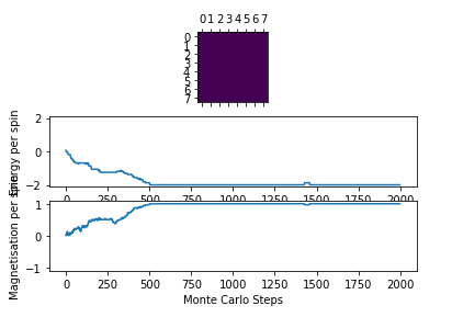Figure 3: Test result @ 1 K
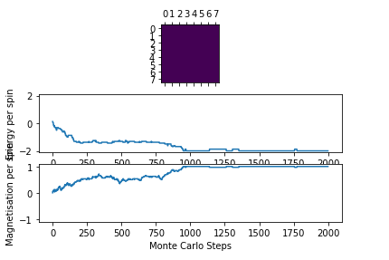Figure 4: Test result @ 1.5 K

The definitions of two class functions were changed as shown below to accommodate this change.

    def montecarlostep(self, T):
        # complete this function so that it performs a single Monte Carlo step
        energy = self.energy()
        #the following two lines will select the coordinates of the random spin for you
        random_i = np.random.choice(range(0, self.n_rows))
        random_j = np.random.choice(range(0, self.n_cols))
        #the following line will choose a random number in the range [0,1) for you
        random_number = np.random.random()
        self.lattice[random_i][random_j] = -self.lattice[random_i][random_j]
        energy2 = self.energy()
        dE = energy2 - energy

        if energy2<energy or random_number<=np.e**(-(energy2-energy)/T):
            yyy=True
        else:
            self.lattice[random_i][random_j] = -self.lattice[random_i][random_j]
			
        self.n_cycles+=1
        if self.n_cycles==1000:
            self.E=0
            self.E2=0
            self.M=0
            self.M2=0
        self.E += self.energy()
        self.E2 += self.energy()**2
        self.M += self.magnetisation()
        self.M2 += self.magnetisation()**2
        return self.energy(), self.magnetisation()

    def statistics(self):
        # complete this function so that it calculates the correct values for the averages of E, E*E (E2), M, M*M (M2), and returns them
        avE = self.E / self.n_cycles
        avE2 = self.E2 / self.n_cycles
        avM = self.M / self.n_cycles
        avM2 = self.M / self.n_cycles
        if self.n_cycles>1000:
            avE = self.E / (self.n_cycles-1000)
            avE2 = self.E2 / (self.n_cycles-1000)
            avM = self.M / (self.n_cycles-1000)
            avM2 = self.M / (self.n_cycles-1000)
        return avE, avE2, avM, avM2, self.n_cycles

Range of temperatures

The experiment was run for 8x8 lattice at a temperature range of 0.25 K-5.00 K, with a point every 0.05 K. The experiments using a different number of total steps were performed and the comparison is shown below in figures 5-7.

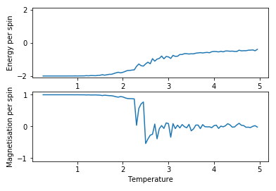Figure 5: Test result for 8x8 lattice with 11000 steps
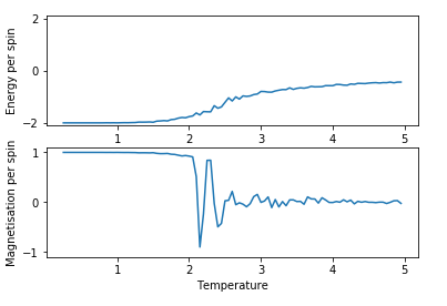Figure 6: Test result for 8x8 lattice with 21000 steps
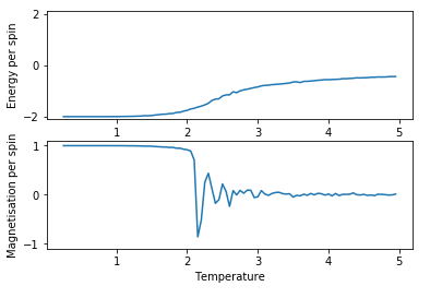Figure 7: Test result for 8x8 lattice with 101000 steps

There is a small, but noticeable improvement in the smoothness of the curves obtained for energy with using more steps, thus the highest number of steps (101000 steps) was used in the further experiments regardless of the higher need for computational power.

Lattice size effects

With increasing lattice size the energy and magnetisation curves become more realistic, since the long range effects are better accounted for. 7 different lattice sizes were tested and energy and magnetisation for each are shown below in figure 8-14 and 15-21 respectively.

Figure 8: Energy result for 2x2 lattice
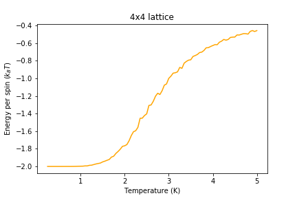Figure 9: Energy result for 4x4 lattice
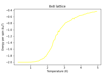Figure 10: Energy result for 8x8 lattice
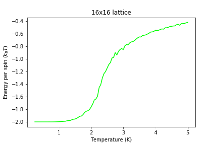Figure 11: Energy result for 16x16 lattice
Figure 12: Energy result for 32x32 lattice
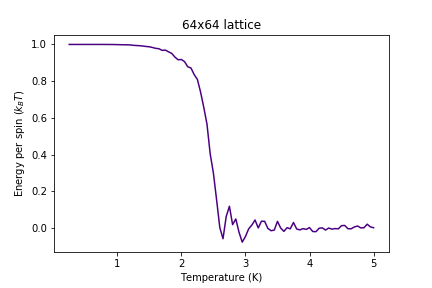Figure 13: Energy result for 64x64 lattice
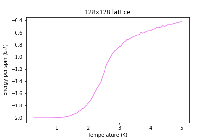Figure 14: Energy result for 128x128 lattice
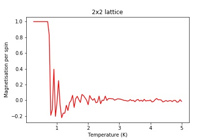Figure 15: Magnetisation result for 2x2 lattice
Figure 16: Magnetisation result for 4x4 lattice
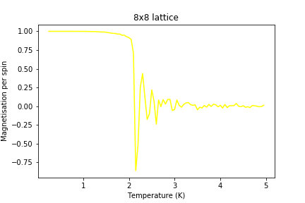Figure 17: Magnetisation result for 8x8 lattice
Figure 18: Magnetisation result for 16x16 lattice
Figure 19: Magnetisation result for 32x32 lattice
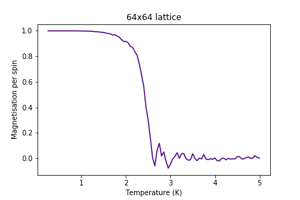Figure 20: Magnetisation result for 64x64 lattice
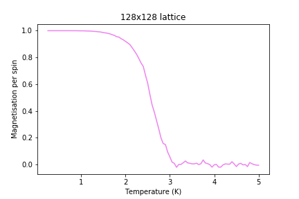Figure 21: Magnetisation result for 128x128 lattice

Overall comparison of energy and magnetisation per spin in each lattice was made and can be seen in figures 22 and 23 below.

Figure 22: Energy comparison
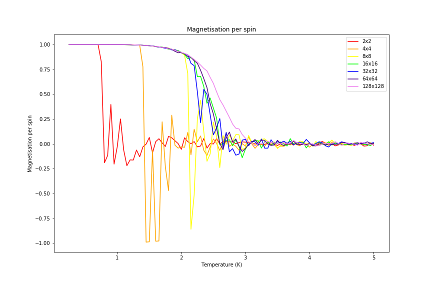Figure 23: Magnetisation comparison

The code used for producing figure 23 above is shown below. Other codes are analagous. Example for defining ls2 is also shown Others are similar..

ls2=loadtxt("2x2(100).dat")

figsize(12,8)
plot(ls2[:,0],ls2[:,3]/4,color="red",label="2x2")
plot(ls4[:,0],ls4[:,3]/16,color="orange",label="4x4")
plot(ls8[:,0],ls8[:,3]/64,color="yellow",label="8x8")
plot(ls16[:,0],ls16[:,3]/256,color="lime",label="16x16")
plot(ls32[:,0],ls32[:,3]/1024,color="blue",label="32x32")
plot(ls64[:,0],ls64[:,3]/4096,color="indigo",label="64x64")
plot(ls128[:,0],ls128[:,3]/16384,color="violet",label="128x128")
title("Magnetisation per spin")
xlabel("Temperature (K)")
ylabel("Magnetisation per spin")
legend()
savefig("Magnetisation.png")
show()

Significant changes may be observed from 2x2 lattice up to 16x16 lattice, later the additional long range effects become less noticeable, but new effects are still present. It seems that most of the long range effects are captured by 16x16 lattice, but higher dimensions bring additional improvement.

Heat Capacity

This formula holds true by definition: $C = \frac{\partial ⟨ E ⟩}{\partial T}$ .

Variance of energy can be calculated in the following way: $V a r [X] = ⟨ E^{2} ⟩ - {⟨ E ⟩}^{2}$ .

Since expected energy can also be expressed as partition function: $⟨ E ⟩ = \frac{\partial}{\partial β} l n Z$ , variance may be expressed as $V a r [X] = \frac{\partial^{2}}{\partial β^{2}} l n Z = - \frac{\partial ⟨ E ⟩}{\partial β}$ .

We can rearrange the equations given, because $T = \frac{1}{k_{B} T}$ , so that we obtain $C = \frac{V a r [E]}{k_{B} T^{2}}$ .

Heat capacity of the model

Heat capacities of the models were calculated using the script given below (example for 2x2 lattice).

figsize(6,4)
plot(ls2[:,0],(ls2[:,2]-ls2[:,1]**2)/ls2[:,0],color="red",label="2x2")
xlabel("Temperature (K)")
ylabel("C")
savefig("C2.png")
show()

Graphs of heat capacities are shown in the gallery below (figures 24-30). It can be seen that the model breaks down at low temperatures for bigger lattices, but it still gives a peak heat capacity.

Figure 24: C result for 2x2 lattice
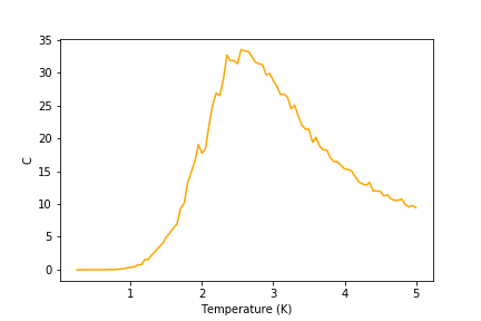Figure 25: C result for 4x4 lattice
Figure 26: C result for 8x8 lattice
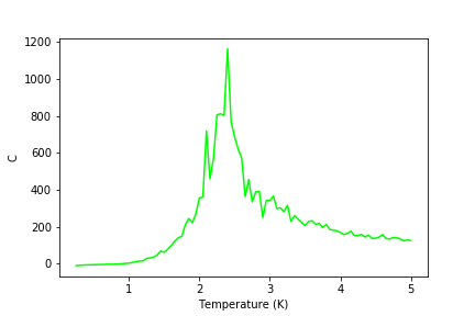Figure 27: C result for 16x16 lattice
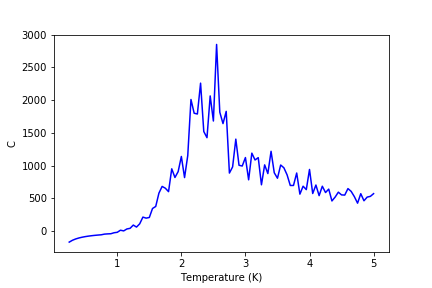Figure 28: C result for 32x32 lattice
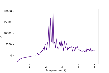Figure 29: C result for 64x64 lattice
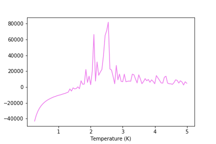Figure 30: C result for 128x128 lattice

Comparison of heat capacity per spin is given in the figure 31 below.

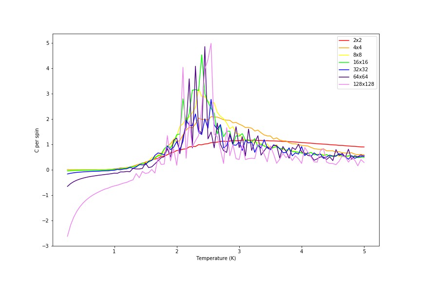Figure 31: Heat capacity comparison

Curie temperature

Curie temperature can be deduced from where there is a peak in heat capacity per spin. The graphs of heat capacity vs temperature is shown below (figures 32 and 33) for two different lattice sizes, once using Python script and once using C++ data provided.

Figure 32: 16x16 lattice
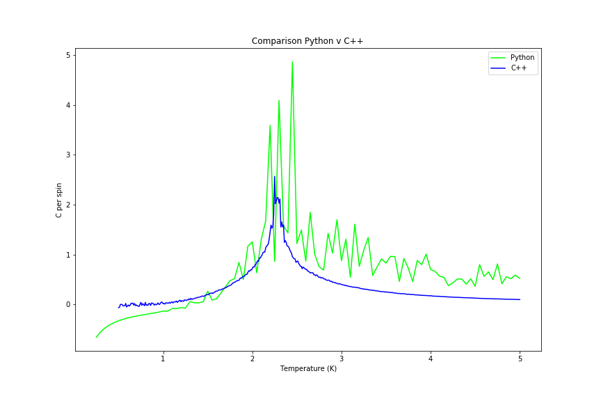Figure 33: 64x64 lattice

Polynomial fit

The C++ data was also fitted with a polynomial, firstly over the whole range and afterwards just in the peak range. Fitting a polynomial proved to be hard as expected (since data is close to delta-like function), but it became more feasible when smaller range was used. Examples of both fits are shown in figures 34 and 35 below.

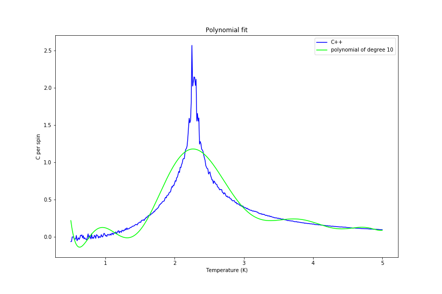Figure 34: Whole region fit
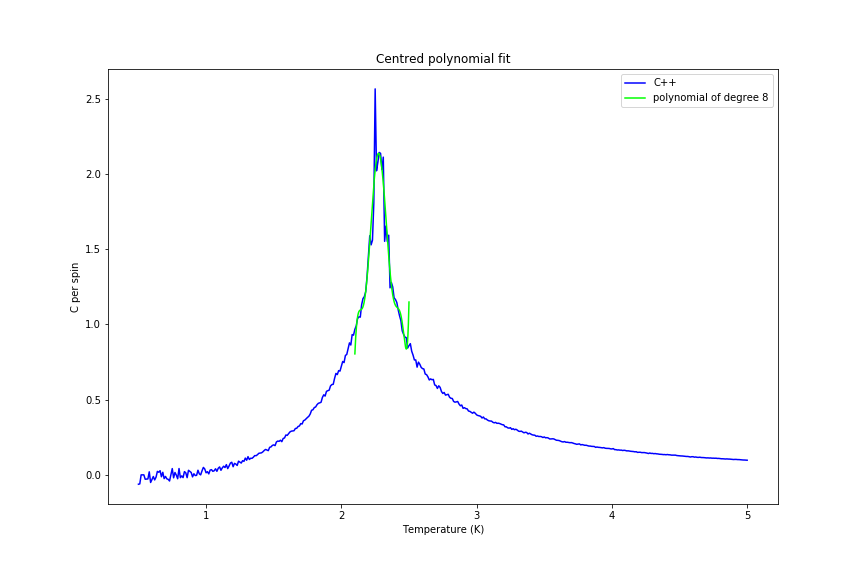Figure 35: Peak region fit

Finding Curie temperature

The last step was to find peak heat capacity for different lattice sizes in C++ data. The results are shown in the table below.

Lattice size	Curie temperature
2x2	2.48 K
4x4	2.40 K
8x8	2.32 K
16x16	2.25 K
32x32	2.30 K
64x64	2.25 K

The curie temperature for infinite lattice is known to be calculated from that of a finite lattice using equation $T_{C, L} = \frac{A}{L} + T_{C, \infty}$ , where $T_{C, L}$ is the Curie temperature of an $L \times L$ lattice, $T_{C, \infty}$ is the Curie temperature of an infinite lattice, and $A$ is a constant. This was used to draw a graph shown in figure 36 below.

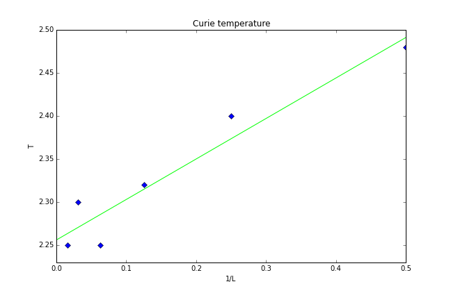Figure 36: Curie temperature for infinite lattice

The Curie temperature for infinite lattice was found to be $T = 2.26 K$ .

The code used for drawing the graph in figure 36 is shown below.

L=array([1/2,1/4,1/8,1/16,1/32,1/64])
T=array([2.48,2.4,2.32,2.25,2.3,2.25])
X=array([1/2,0])
figsize(9,6)
plot(L,T,marker="D",linestyle=" ")
xlabel("1/L")
ylabel("T")
a=polyfit(L,T,1)
ylim(2.23,2.5)
plot(X,a[0]*X+a[1],color="lime")
title("Curie temperature")
savefig("Curie.png")
show()