Rep:CMPY3:OPB16
Ising Model of a Ferromagnet Described Using Monte Carlo Simulations
Oliver Burman, CID: 01220361, 21st November 2018
Abstract
Simulations were run for 2D Ising Models of ferromagnets using a Metropolis Monte Carlo algorithm to find the lattice with the lowest free energy at a given temperature. This is determined by the competition of energy minimisation and entropy maximisation. In the 2D Ising model, a LxL lattice is created with each cell having a +1, or -1 spin, the interactions of this cell with its nearest neighbours determines the interaction energy of the lattice. The Monte Carlo method works by changing a random spin in the lattice and seeing if this change is energetically beneficial to the system. In this experiment 2x2, 4x4, 8x8, 16x16 and 32x32 lattices are used to determine heat capacities () and locate each lattice's Curie Temperature (). Since this experiment is simulating a ferromagnetic lattice, the Curie Temperature is the temperature at which the ferromagnetic properties are lost and the system becomes paramagnetic, resulting in a total magnetisation equal to zero. The Curie reduced temperature for an infinite lattice was calculated to be 2.19.
Introduction to the Ising Model
The Model
The Ising model replicates a ferromagnet by creating a lattice of spins that are either +1 or -1. Each spin or cell interacts with its nearest neighbours to generate an energy for the whole lattice. The interaction energy of the lattice is shown by the equation below:
(1)
where is the spin of cell i and spin j are from cells that are nearest neighbours to i and J is a measure of the strength of interaction between spins. In any system, each cell has 2D nearest neighbours where D is the dimension. In 1D, each cell will interact with two others, in 2D each cell will interact with four (above, below, left and right) and in a 3D lattice there are 6 nearest neighbours. The minimum energy occurs when all spins in the lattice are parallel, either all +1 or all -1. This means that to minimise the energy, the energy between each cell with its nearest neighbour will be which will be 1. Since each cell, i interacts with 2D neighbours, the interaction energy per cell is 2D:
And since there are N cells, there are N times this energy:
× (2)
Regardless of the the number of spins in the lattice (N), the multiplicity of this low energy state is 2. This is because both an entire lattice of all spin +1 and all spin -1 are isoeneregetic. This only holds in the absence of an external magnetic field as this would split the two levels.
Using the following equation for entropy:
(3)
Since the multiplicity (Ω) is 2, the entropy is:
×
The magnetisation of the Ising Lattice the sum of every spin in the lattice:
(4)
Phase Transitions
For a D = 3, N = 1000 system, if a single spin is flipped from the minimum energy structure then the new energy is given by the equation below:
(5)
This gives E = -2988J which gives and energy change, ΔE = -12J. The first term gives the interaction energy from the spins whose interactions are unaffected by the flip. The second term is the interactions of the spin that has flipped interacting with its 2D nearest neighbours. And the final term accounts for the interactions of those nearest neighbours that are affected by the flip. As mentioned before, there are only two configurations in the lowest energy state (all spin up or all spin down). After a single flip there are 2,000 possible configurations as the flipped cell could be any of the N = 1000 cells, and there are two possible lattices (999 spin-up or 999 spin-down). This gives the following entropy change:
×
 |
From figure 1, the D = 1; N = 5 lattice has 3 x +1 spins and 2 x -1 spins. This gives . And the D = 2; N = 5x5, has 13 positive spins and 12 negative spins giving also.
For a D = 3, N =1000 Isling lattice at absolute zero, it is expected that the lattice will adopt the lowest energy structure of having entirely parallel spins, this leads to a or as they are isoenergetic.
Calculating the energy and magnetisation
Modifying the Files
Functions energy() and magnetisation() were made using the equations (1) and (4) in order to calculate the total energy and magnetisation of the lattice. The magnetisation function is simple as it merely adds all spins in the lattice together. The energy function is for a 2D lattice and multiplies a cell's spin with those of its nearest neighbours, this is summed for every cell in the lattice.
def energy(self):
    energy = 0
    "Return the total energy of the current lattice configuration."
    for i in range(self.n_rows):
        for j in range(self.n_cols):
            energy = energy - (self.lattice[i][j]*self.lattice[(i-1)][j])
            - (self.lattice[i][j]*self.lattice[i][(j-1)])
    return energy

def magnetisation(self):
    "Return the total magnetisation of the current lattice configuration."
    mag = np.sum(self.lattice)
    return mag
Testing the Files
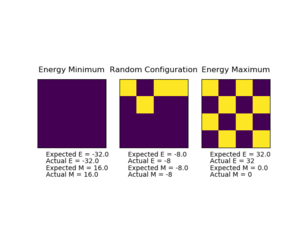 |
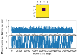
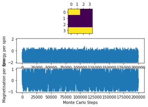
Figure 2 shows the output from running ILcheck.py. The three different 4x4 Isling Lattices show their energies and magnetisations. As the magnetisation per spin is closer to 1 (total magnetisation = 16), the energy is lower since parallel spins are the most energetically stable configuration. For a total of 16 particles in 2D, the minimum energy matches that of equation (2) with a result of -32 which is -2 per spin. The intermediate energy lattice has regions of parallel spins, and the highest energy has zero magnetisation as the spins cancel one another out and lowest energy has completely parallel spins.
Introduction to the Monte Carlo simulation
The average magnetisation and energy of a system are given in statistical mechanics by the following equations:
(6)
(7)
Where represents all the spins in the system and is the partition function.
A system with 100 spins has 2100 possible configurations (with the 2 coming from the spin being either up or down). This is 1.2676506 x 1030 configurations. If a computer could run 1 x 10⁹ configurations s-1, then it would take 1.2676506 x 121 s or 4.019693684 x 10¹³ years (not counting for leap days which is five magnitudes older than the age of the universe.[1] This means that calculating the mean properties using these equations is not a viable method to simulate ferromagnetism.
Instead this experiment will use a Metropolis Monte Carlo algorithm that begins with a 2D Ising lattice of a particular size and at a particular temperature where all the spins in the lattice are random. From this initial configuration, a single random spin is flipped, the energy of this new configuration is calculated and compared to the energy of the initial configuration. If this new energy is less than the original one (), then the flip has energetically benefited the system and the new configuration is accepted. If the new energy is larger than the original (), a random number, is generated in the interval [0,1). if:
then the new configuration is accepted, but if:
then the configuration remains as it did originally, and the spin doesn't flip. After this the averages for the properties of the system are updated and another Monte Carlo cycle will begin. From the relationship between the random number and the Boltzmann factor, it is clear that there is more chance of a random number being large enough to flip the spin for lattices at high temperatures and where the energy change of flipping isn't too large.
The statistics() function returns the average and values per number of Monte Carlo cycles of a lattice.
    def montecarlostep(self, T):
        "Function to run a stepwise Monte Carlo simulation"
        energy = self.energy()
        magnetisation = self.magnetisation()
        random_i = np.random.choice(range(0, self.n_rows))
        random_j = np.random.choice(range(0, self.n_cols))
        self.lattice[random_i,random_j] = -self.lattice[random_i,random_j]
        dE = self.energy() - energy
        if dE > 0:
            if np.random.random() > np.exp(-dE/T):
                self.lattice[random_i,random_j] = -self.lattice[random_i,random_j]
        self.E = self.E + self.energy()
        self.E2 = self.E**2+ self.energy()**2
        self.M = self.M + self.magnetisation()
        self.M2 = self.M**2 + self.magnetisation()**2
        self.n_cycles = self.n_cycles + 1
        return(self.energy(), self.magnetisation())
    def statistics(self):
        "Function that return the average E, E^2, M and M^2 per spin for the lattice"
        avE = self.E/ self.n_cycles
        avE2 = self.E2/ self.n_cycles
        avM = self.M/ self.n_cycles
        avM2 = self.M2 / self.n_cycles
        return(avE, avE2, avM, avM2, n_cycles)
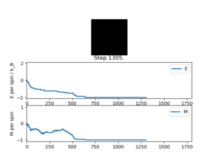 |
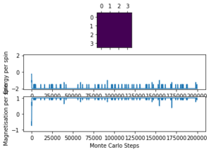
Running ILanim.py gives the output of figure 3 and the numbers below from the statistics() function.
E = -1.661, E*E = 2.9958, M = -0.786, M*M = 0.6994
It can be seen that it takes roughly 600 cycles for both the energy and magnetisation to equilibrate. The average energy per spin converges to the most stable possible value of -2 () and the magnetisation per spin converges to -1 where all the spins in the lattice are parallel. However, these are not the numbers given by the statistics() function, since this records the averages over all of the cycles, including those before the system has equilibrated so does not give accurate data for the equilibrated lattice.
The Curie Temperature, is the temperature at above which materials lose their permanent magnetic properties. For a ferromagnetic material, above the spins are no longer aligned, leaving a disordered, paramagnetic material. This is because of the competition between energy minimisation and entropy maximisation which are both used to minimise the free energy of the system. At higher temperatures the entropy term dominates, as seen by equation (3), this is maximised when there are more possible configurations in the lattice. At lower temperatures the entropy is less significant and thus the internal energy is minimised. The turning point for this is the phase transition is at . For it is expected that once the lattice equilibrates, all spins should be aligned and thus a non-zero magnetisation. An equation that shows the competition between energy minimisation and entropy maximisation to dominate the free energy is shown below:
(8)
where is the Helmholtz free energy, is the internal energy that is maximised by decreasing the interaction energy between each spin and is the entropy which is made more relevant in the equation at higher values of .
Accelerating the code
In order to decrease the computing time required for a simulation, the efficiency of the code is increased. This is done by reducing the number of loops used in the code. The magnetisation function is already optimised, however, using np.sum, np.multiply and np.roll functions from numpy (np), the efficiency for calculating the energy is increased. The optimised code for the energy is shown below.
    def energy(self):
        "Return the total energy of the current lattice configuration."
        energy = -np.sum(np.multiply(self.lattice, np.roll(self.lattice,(1,0))))
        -np.sum(np.multiply(self.lattice, np.roll(self.lattice,(1,1))))
        return energy
Here the np.roll function is used to shift the lattice to find the nearest neighbours of each cell.
ILtimetrial.py was run to record the time taken to run 2,000 Monte Carlo steps. This was used for both the original and optimised code with a standard error being calculated from the repeat reading. Before it took 6.616 ± 0.035 s and after only 0.523 ± 0.001 s. This shows that the addition of the numpy functions into the energy function has greatly reduced the computing time for the simulation allowing for more time efficient simulations to be run. This is very significant since some simulations run 250,000 cycles per temperature step, and 95 temperature steps over a range are used.
The effect of temperature
Currently the statistics function is calculating average values for and per cycle using the energy from all cycles run. These values only want to be recorded for the lattice once it has equilibrated for further calculations. For this reason, the initial cycles of the simulation want to be discarded such that the energy and other properties only begin to be recorded when the lattice has equilibrated. This was done by editing the code for the montecarlostep() and statisitics() functions:
    def montecarlostep(self, T):
        "Function to perform a Monte Carlo step"
        energy = self.energy()
        magnetisation = self.magnetisation()
        sample_size = 150000
        random_i = np.random.choice(range(0, self.n_rows))
        random_j = np.random.choice(range(0, self.n_cols))
        self.lattice[random_i,random_j] = -self.lattice[random_i,random_j]
        dE = self.energy() - energy
        if dE > 0:
            if np.random.random() > np.exp(-dE/T):
                self.lattice[random_i,random_j] = -self.lattice[random_i,random_j]

        self.n_cycles = self.n_cycles + 1
        if self.n_cycles >= sample_size:
            self.E  += self.energy()
            self.E2 += self.energy()**2
            self.M  += self.magnetisation()
            self.M2 += self.magnetisation()**2
            self.N_cycles = self.N_cycles + 1
    def statistics(self):
        "Function that return the average E, E^2, M and M^2 per spin for the lattice"
        avE = self.E/ self.N_cycles
        avE2 = self.E2/ self.N_cycles
        avM = self.M/ self.N_cycles
        avM2 = self.M2 / self.N_cycles
        N_cycles = self.N_cycles
        return(avE, avE2, avM, avM2, N_cycles)
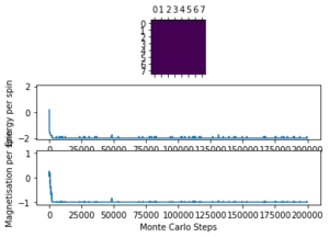
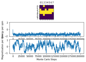
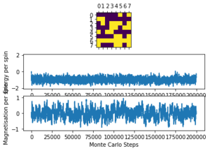
The altered code now introduces "sample_size" and "N_cycles" into the Monte Carlo step. The first of these is the number of initial cycles that are ignored, this removes these cycles from the calculations in statistics. Once the number of cycles (n_cycles) reaches this 'sample_size", and begin to be recorded and the number of cycles they are recorded and averaged over are labelled as "N_cycles". The value of "sample_size" is determined using the output of the ILfinalframe.py script (figures 4 - 11). This script runs similar to ILanim.py but only gives a picture of the equilibrated structure. Examining the 8x8 plots, at lower temperatures the model adopts the energetically stable configuration where the magnetisation per spin = 1 and energy per spin = -2. As the temperature increases, the equilibrated state of the lattice no longer has completely aligned spins, meaning that the Curie Temperature has been crossed. As the temperature increases, the plots have larger noise due to increased thermal fluctuations.
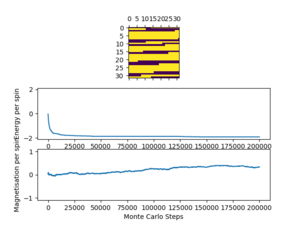 |
For the 8x8 system at small temperatures, it only takes a couple of thousand cycles to equilibrate, however, it is hard to spot at larger temperatures due to the aforementioned thermal fluctuations. Because of this a larger "sample_size" value of 100,000 cycles is chosen to make sure that only equilibrated values are counted. Since the computational time for the smaller lattices (2x2, 4x4, 8x8) is quite small, it is not issue to run the lattice for a larger number of cycles than necessary to make sure that all unwanted cycles are ignored.
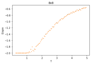
Using 150,000 cycles and recording only the last 50,000 ('sample_size" = 100,000), the ILtemperaturerange.py is run to display the energy and magnetisation of the equilibrated lattice at different temperatures. To make sure the transition between ferromagnetic and paramagnetic is observed, temperatures between T = 0.25 an 5.00 are used. Initially a temperature step, dT of 0.1 was used. However, this did not give a good enough resolution of the system in the energy and magnetisation versus temperature plots. This is mainly an issue when examining the transition period which can be quite short and thus requiring a small enough dT to be accurately displayed. For this reason, a temperature step of 0.05 is chosen. A 0.01 temperature step was attempted, however, it was not worth the additional computational time, especially for larger lattice sizes that can take multiple hours to run. The energy and magnetisation per spin versus temperature plots for the 8x8 lattice are shown in figures 13 and 14 respectively. The error-bars are calculated using the standard error of the data and are therefore very small since each value is recorded over 50,000 cycles. There is and increase in the errors at higher temperatures for the average energy due to thermal fluctuations, and the errors are largest around the transition temperature for the average magnetisation as the magnetisation rapidly fluctuates between positive and negative values.
 |
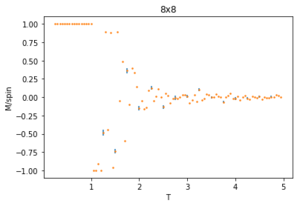 |
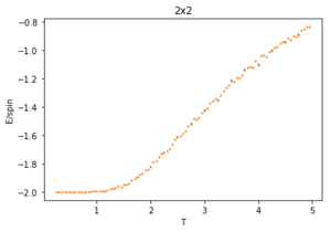
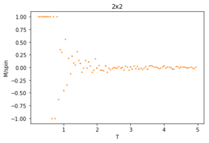
The energy plot starts at the expected average per spin of -2 then drastically increases over the temperature range 1.25 - 4 before smoothing off to an average energy of approximately -0.6. This can be explained by looking at the magnetisation plot. The average magnetisation begins at +1 where all the spins are aligned but this also changes drastically over the same aforementioned temperature range till it smooths off to a value of 0. This signifies that the total magnetisation of the system is 0 and thus the lattice is now paramagnetic, having disordered spins to maximise the entropy and not minimising the internal energy.
The effect of system size
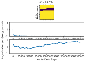
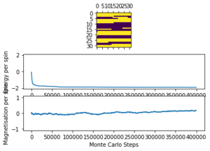
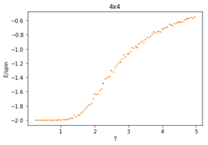
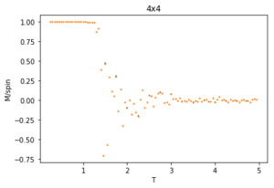
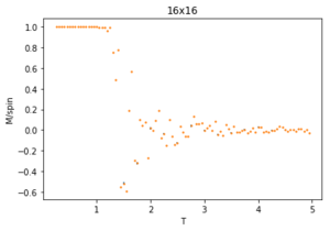
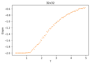
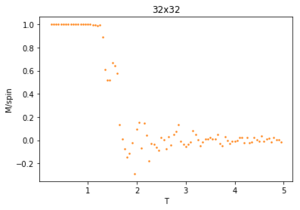
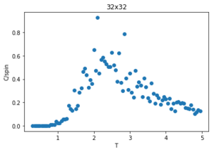
The ILtemperaturerange.py script is run using 2x2, 4x4, 16x16 and 32x32 lattice sizes as well. Approximate guesses for the "sample_size" of each lattice is done by the same way of looking at when each lattice equilibrates at different temperatures in figures 4-12. As stated before the computation time for small lattices is small in comparison to that of the larger lattices so for 2x2, 4x4 and 8x8 systems, a 150,000 cycle simulation is run where the last 50,000 cycles are used to record the properties of the system which more than removes the equilibration cycles. For 16x16 and 32x32 outputs such as figure 11 show it can take upwards of 150,000 for the magnetisation to converge even though the energy converges much faster, making the magnetisation equilibration time the limiting factor. Since these larger lattices take longer equilibrate, 250,000 cycles are run and with the last 50,000 cycles being used. Even at low temperatures these larger lattices can equilibrate to structures where not all of the spins are aligned. This can be seen explicitly in the case where a 32x32 lattice is run at T = 0.05 (figure 11). The reason for this is that in large lattices there are more metastable states which are not easy to escape from as a single spin flip from the Monte Carlo algorithm does not give enough of a perturbation to move the total energy out of the deep well towards the global minimum. All these simulations are run using the same 0.05 temperature step and T = 0.25 - 5 range as before and are given by figures 15 to 22.
As before, the error bars are very small due to the standard error being calculated over 50,000 cycles per temperature step but do increase with increasing T due to the thermal fluctuations. The fluctuations in magnetisation around the Curie Temperature require a smaller temperature step to be more accurately understood. For the 32x32 lattice these fluctuations are not properly captured as they are much too smooth for rapid changes in magnetisation where as they are too sharp, going up to the maximum values of +1 and -1 many times for 8x8 lattices and smaller. This is due to the smaller lattices not being large enough to capture the fluctuations, but the 32x32 lattice being too large to be properly sampled. Because of this 16x16 is the ideal lattice to observe long range fluctuations out of those created for this experiment, but more lattices should be generated between L = 8 and 32 to determine the ideal maximum and minimum lattice sizes to observe these fluctuations.
Determining the heat capacity
The specific heat capacity of a system is defined as:
(9)
where is equivalent to the internal energy of the system, . The variance of the internal energy is equivalent to the rate of change in internal energy with respect to thermal fluctuations, where :
(10)
Using the chain rule:
(11)
This can also be shown by differentiating the following statistical mechanics equation for energy:
(12)
(13)
×
(14)
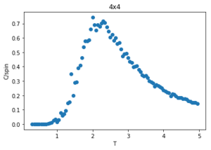
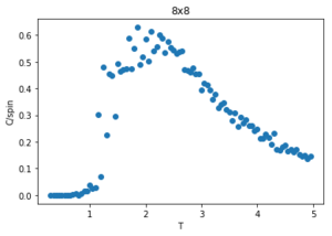
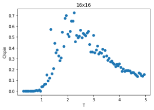
Figures 23-27 show the heat capacity, against temperature for each lattice size. As the lattice size increases, the plot becomes broader, less like a sharp peak. For these larger systems, better resolutions are required and thus smaller time steps needed. It is much harder to accurately sample a system of 1024 cells with 21024 possible configurations (32x32) than it is a system with only 4 lattices and 24 possible configurations (2x2). The peak of these graphs should correspond to when = , however due to the noise surrounding these peaks, especially for large L, it is hard to determine where the maximum value should be.
 |
Locating the Curie temperature
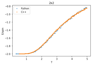
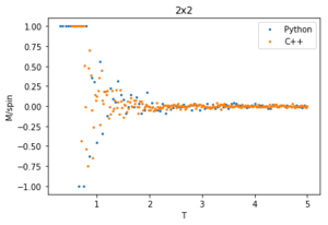
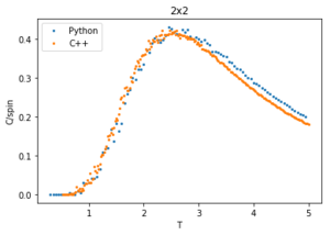
The data from this experiment is compared with that collected using a C++ Monte Carlo algorithm run over a longer period on more powerful computer and an example is displayed in figures 28-30 for 2x2 lattices. The C++ code runs a lot faster making a smaller temperature step more viable, it uses a 0.01 dT whereas the python code is using a 0.05 dT so the C++ has a much better resolution by having more data points within the temperature region. For this 2x2 lattice the two sets of data match very well for all calculated properties, however at higher temperatures the peak of the vs peak is smaller than that in the C++ plot. Since the heat capacity peak is very noisy for the larger lattices, the python data is not resolved enough to perfectly capture the detail around this point. This is of no consequence to future calculations though, as the numerical values of are of no significance since for an infinite lattice the peaks should go to infinity, only the temperature at which occurs, which does match with that of the C++ data.
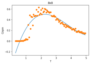
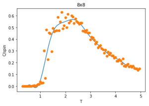
To correct for the issue with large noise surrounding the peak of the vs. plots in the previous section, the polyfit() function is used to fit each curve and then a maximum heat capacity, can be determined leading to the correlating Curie Temperature of a given lattice size. The polynomial order of the polyfit() can be varied to give different fits to the curve. An example of this can be seen in figures 30-32 where the higher order polynomials give a better fit to the actual curve.
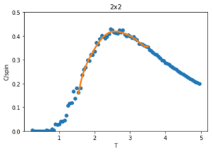
Since only the data surrounding the phase transition temperature is needed, the fit of the data is enhanced by fitting the curve within this transition region. An example of this is shown in figure 34 for a 2x2 lattice. The temperatures corresponding to max specific heat capacity values of the fit for each lattice size () are calculated and given below:
| L | 1/L | TC,L |
|---|---|---|
| 2 | 0.5 | 2.6 |
| 4 | 0.25 | 2.3 |
| 8 | 0.125 | 2.25 |
| 16 | 0.0625 | 2.2 |
| 32 | 0.03125 | 2.3 |
With the exception of L = 32, the general trend is that the Curie Temperature decreases with increasing lattice size. The 32x32 may be giving a value higher than expected due to the simulation not being able to fully sample the large system as mentioned before. This data is then used to calculate the Curie Temperature for an infinite lattice, using the equation:
(15)
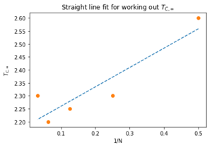 |
A polyfit() is created to generate a straight line based on this equation. This plot is given in figure 35 and it has a gradient of 0.746 and an intercept on the axis of 2.185. These numbers relate to (a constant of the lattice) and respectively. The standard deviation associate with this Curie Temperature is 0.0078. In 1944, Lars Onsager solved the 2D Ising Lattice to give the following : [2]
- (16)
Here the Boltzmann factor and interaction strength constant are shown, where as in our model the temperature is already normalised to and is taken as 1. This value is only 0.084 away from the one calculated in this experiment. This is not within the standard deviation but considering the issues with our code for larger lattices, the two infinite length Curie Temperatures are very close.
Conclusion
The Monte Carlo algorithm created for this experiment has worked very well, leading to a Curie Temperature for an infinite lattice (2.19) close to that calculated in literature. The energy and magnetisation averages also matched closely with data generated from a much more powerful C++ script. The main issues with the algorithm was that it was too slow running using python so a smaller temperature step couldn't be used, and that it began to fail at larger lattice sizes. A smaller dT would have led to a greater resolution of the simulation and may have improved the results obtained for the larger lattices. Since the 32x32 had many more spins than the other lattices, the code struggled to sample it all accurately. As there is such a larger increase in number of spins from an L = 16 to L = 32 more intermediate lattice sizes should have been investigated. This would have given more lattices that are suitable for observing long range fluctuations since the 8x8 lattice was too small to capture this and the 32x32 was not sampled well enough to see them. It also would have improved the fit for the straight line used to determine as only five lattice sizes were recorded, and five is the minimum number of data points required for a polyfit().
Code
Complete Isinglattice.py
import numpy as np

class IsingLattice:

    def __init__(self, n_rows, n_cols):
        self.n_rows = n_rows
        self.n_cols = n_cols
        self.lattice = np.random.choice([1,-1], size=(n_rows, n_cols))
        self.E = 0
        self.E2 = 0
        self.M = 0
        self.M2 = 0
        self.n_cycles = 1
        self.N_cycles = 1

    def energy(self):

        "Return the total energy of the current lattice configuration."

        energy = -np.sum(np.multiply(self.lattice, np.roll(self.lattice,(1,0))))-np.sum(np.multiply(self.lattice, np.roll(self.lattice,(1,1))))

        return energy

    def magnetisation(self):
        "Return the total magnetisation of the current lattice configuration."
        mag = np.sum(self.lattice)
        return mag

    def montecarlostep(self, T):
        "Completes a Monte Carlo step"
        energy = self.energy()
        magnetisation = self.magnetisation()


        sample_size = 150000
        #this is the cut-off point for n_cycles

        random_i = np.random.choice(range(0, self.n_rows))
        random_j = np.random.choice(range(0, self.n_cols))
        self.lattice[random_i,random_j] = -self.lattice[random_i,random_j]
        dE = self.energy() - energy
        if dE > 0:
            if np.random.random() > np.exp(-dE/T):
                self.lattice[random_i,random_j] = -self.lattice[random_i,random_j]

        self.n_cycles = self.n_cycles + 1


        if self.n_cycles >= sample_size:
            self.E  += self.energy()
            self.E2 += self.energy()**2
            self.M  += self.magnetisation()
            self.M2 += self.magnetisation()**2
            self.N_cycles = self.N_cycles + 1
            #N_cycles are the cycles used for averaging and the cycles that data is recorded over

        return(self.energy(), self.magnetisation())


    def statistics(self):
        "Returns the correct values for the averages of E, E*E (E2), M, M*M (M2)"
        avE = self.E/ self.N_cycles
        avE2 = self.E2/ self.N_cycles
        avM = self.M/ self.N_cycles
        avM2 = self.M2 / self.N_cycles
        N_cycles = self.N_cycles

        return(avE, avE2, avM, avM2, N_cycles)
Example code for reading a 2x2.dat file (for other files change 2 to 4, 8, 16 etc.):
import numpy as np
%pylab inline
t2 = np.loadtxt('2x2.dat')
#importing the data file
t2c = np.loadtxt('2x2C.dat')
#importing the C++ data file
T2 = t2[:,0]
E2 = t2[:,1]
E22 = t2[:,2]
M2 = t2[:,3]
M22 = t2[:,4]

T2c = t2c[:,0]
E2c = t2c[:,1]
E22c = t2c[:,2]
M2c = t2c[:,3]
M22c = t2c[:,4]
C2c = t2c[:,5]
#labelling each column in the files with a property

E2p = E2/2**2
M2p = M2/2**2
#energy and magnetisation per spin

var2 = E22 - (E2)**2
var2 = var2/ 2**2
#variance in E per spin

varm2 = M22 - (M2)**2
varm2 = varm2/2**2
#variance in M per spin

std2 = var2**0.5
se2 = std2/ (50000)**0.5
#standard error in E

stdm2 = varm2**0.5
sem2 = stdm2/ (50000)**0.5
#standard error in M
#plotting E/spin vs T

errorbar(T2[::5], E2p[::5], marker='', linestyle='', yerr=se2[::5])
title('2x2')
xlabel('T')
ylabel('E/spin')
plot(T2, E2p, linestyle = '', marker = 'o', markersize = '1.5')
show()
#plotting M/spin vs T

stdm2 = varm2**0.5
sem2 = stdm2/ (50000)**0.5
#standard error in M
errorbar(T2[::5], M2p[::5], marker='', linestyle='', yerr=sem2[::5])
plot(T2, M2p, linestyle = '', marker = 'o', markersize = '1.5')
title('2x2')
xlabel('T')
ylabel('M/spin')
show()
#plotting C/spin vsT T

var2 = E22 - (E2)**2
C2 = var2/ T2**2
C2p = C2/ 2**2
plot(T2[1:],C2p[1:], linestyle = '', marker = 'o')
ylabel('C/spin')
xlabel('T')
title('2x2')
show()
Comparisons with C++ data
#plotting C vs T
plot(T2[1:],C2p[1:], label = 'Python', linestyle = '', marker = 'o', markersize = '2')
plot(T2c[1:],C2c[1:], label = 'C++', linestyle = '', marker = 'o', markersize = '2')
legend(loc='upper left')
ylabel('C/spin')
xlabel('T')
title('2x2')
show()
#plotting E vs T

plot(T2[1:],E2p[1:], label = 'Python', linestyle = '', marker = 'o', markersize = '2')
plot(T2c[1:],E2c[1:], label = 'C++', linestyle ='', marker = 'o', markersize ='2')
legend(loc='upper left')
ylabel('E/spin')
xlabel('T')
title('2x2')
show()
#plotting M vs T

plot(T2[1:],M2p[1:], label = 'Python', linestyle = '', marker = 'o', markersize ='2')
plot(T2c[1:],M2c[1:], label = 'C++', linestyle = '', marker = 'o', markersize = '2')
legend(loc='upper right')
ylabel('M/spin')
xlabel('T')
title('2x2')
show()
Using polyfit()
import numpy as np
from matplotlib import pylab as pl
%pylab inline
#import data
data2 = np.loadtxt("2x2.dat")
T2 = data2[:,0]
E2 = data2[:,1]
E22 = data2[:,2]

var2 = E22 - (E2)**2
C2 = var2/ T2**2
C2 = C2/ 2**2

#first we fit the polynomial to the data
fit2 = np.polyfit(T2, C2, 10) # fitted to a tenth order polynomial

#now we generate interpolated values of the fitted polynomial over the range of our function
T_min2 = np.min(T2)
T_max2 = np.max(T2)
T_range2 = np.linspace(T_min2, T_max2, 1000) #generate 1000 evenly spaced points between T_min and T_max
fitted_C_values2 = np.polyval(fit2, T_range2) # use the fit object to generate the corresponding values of C

plot(T_range2, fitted_C_values2)
xlabel('T')
ylabel('C/spin')
title('2x2')
plot(T2, C2)
show()
#fitting around a peak
Tmin2 = 1.5
Tmax2 = 3.5

selection2 = np.logical_and(T2 > Tmin2, T2 < Tmax2) #choose only those rows where both conditions are true
peak_T_values2 = T2[selection2]
peak_C_values2 = C2[selection2]

fit2 = np.polyfit(peak_T_values2, peak_C_values2,7) # fitting to a seventh order polynomial

T_range2 = np.linspace(T_min2, T_max2, 1000)
fitted_C_values2 = np.polyval(fit2, peak_T_values2) # use the fit object to generate the corresponding values of C

plot(T2, C2, linestyle = '', marker = 'o')
plot(peak_T_values2, fitted_C_values2, linewidth = '3')
xlabel('T')
ylabel('C/spin')
title('2x2')

ylim(0,0.5)
show()
Calculating T_{C,inf} assuming pervious two blocks of code have been run for all lattice sizes
C2max = np.max(fitted_C_values2)
T2max = peak_T_values2[fitted_C_values2 == C2max]

C4max = np.max(fitted_C_values4)
T4max = peak_T_values4[fitted_C_values4 == C4max]

C8max = np.max(fitted_C_values8)
T8max = peak_T_values8[fitted_C_values8 == C8max]

C16max = np.max(fitted_C_values16)
T16max = peak_T_values16[fitted_C_values16 == C16max]

C32max = np.max(fitted_C_values32)
T32max = peak_T_values32[fitted_C_values32 == C32max]

Tlist = [T2max, T4max, T8max, T16max, T32max]
Nlist = array([2,4,8,16,32])

p = polyfit(1/Nlist, Tlist, 1, cov=True)
p = p[0]

m=p[0]
c=p[1]
#c, the intercept is T_c_inf, m is A.

fitted = m*(1/Nlist) + c
#fitting to a straight line
plot(1/Nlist, fitted, linestyle='--')
plot(1/Nlist, Tlist, linestyle='', marker = 'o')
xlabel('1/L')
ylabel('$T_{C,L}$')
title('Straight line fit for working out $T_{C,∞}$')
show()

