Rep:CMP:yht17
Section 1
In the Ising model, the total interaction energy , where N is the number of spins, si is the spin of lattice point i and J is a constant for the strength of the interaction.
The lowest energy state is when all the spins are in the same direction. This means that for all i and j.
Each lattice point has 2D neighbours, where D is the number of dimensions. The lowest possible energy using this model is thus .
The multiplicity of this state is 2, since the spins can be all up or all down.
The entropy J K-1.
In a system where D = 3 and N = 1000 and in its lowest energy state, E = -3000J and S = 9.57 × 10⁻²⁴ J K-1.
If one of the spins were to flip, E = -2988J and S = 1.05 × 10⁻²² J K-1. ΔE = 12J and ΔS = 9.54 × 10⁻²³ J K-1.

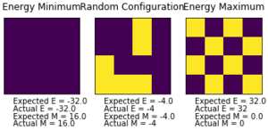
The total magnetisation of a system . In figure 1, the total magnetisation of the 1D and 2D lattices are both 1.
In a lattice with D = 3 and N = 1000 at absolute zero, there is no entropic contribution to the free energy, so all the lattice points should have the same spin and the total magnetisation should be ±1000.
Section 2
Section 3
In a system with 100 spins, there are 2100, or about 1.27 × 1030 possible configurations. If a computer could analyse and find the energy and magnetisation for 109 of these configurations per second, it would take over 40 trillion years to find a single value of .
To accelerate the process, a Monte Carlo algorithm was employed.
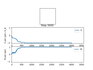
At a temperature below TC, the spins of the entire lattice should align, resulting in magnetisation.
| E | -2.0 |
|---|---|
| E2 | 4.0 |
| M | 1.0 |
| M2 | 1.0 |
The temperature of the simulation in figure 3 is below TC, and indeed the spins do align. The statistics in table 1 also show that the spins are aligned.
Due to issues with the animation script, this part was completed after the statistics function was fixed to account for the time taken to equilibriate.
Section 4
The script to run the Monte Carlo algorithm may not be very fast.
A test function was used to time how long it takes for the script to run a 25 by 25 grid of spins for 2000 steps at T = 1. This was done on a campus computer.
| Trial 1 (s) | Trial 2 (s) | Trial 3 (s) | Trial 4 (s) | Trial 5 (s) | Average (s) | Standard deviation (s) |
|---|---|---|---|---|---|---|
| 2.2466 | 2.2551 | 2.2456 | 2.2509 | 2.2414 | 2.2479 | 0.0021 |
The script was optimised using some built-in functions from the numpy module and the test was repeated.
| Trial 1 (s) | Trial 2 (s) | Trial 3 (s) | Trial 4 (s) | Trial 5 (s) | Average (s) | Standard deviation (s) |
|---|---|---|---|---|---|---|
| 0.2151 | 0.2159 | 0.2220 | 0.2194 | 0.2155 | 0.2176 | 0.0012 |
The optimisation results in a script that is over 10 times faster than the unoptimised script.
| Trial 1 (s) | Trial 2 (s) | Trial 3 (s) | Trial 4 (s) | Trial 5 (s) | Average (s) | Standard deviation (s) |
|---|---|---|---|---|---|---|
| 0.1343 | 0.1349 | 0.1355 | 0.1351 | 0.1356 | 0.1351 | 0.0002 |
With some further optimisations to the algorithm step method, the script is now over 15 times faster than the original unoptimised script.
Section 5
After the beginning of the simulation, there is a period of time before the system reaches equilibrium. This time varies as the temperature and size of lattice changes, but it increases as the lattice size increases and also generally as the temperature decreases. For the average energies and magnetisations to be accurate, they should not take into account any states before the system reaches equilibrium. This can be achieved by manually setting a cutoff point before which no states are considered. For a 8×8 lattice, 2000 cycles is sufficient for the system to reach equilibrium.
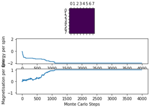
With this fix in place, the script can be used to find properties of the system. By starting with an aligned lattice at a low temperature then repeatedly raising the temperature by a small interval and letting the system equilibriate, the point at which entropy starts to dominate can be found.
Section 6
The simulation was run over the temperature range t = 0.05 to t = 5.0 for the lattice sizes 2×2, 4×4, 8×8, 16×16 and 32×32.
| Lattice size | Cycles | Cutoff point |
|---|---|---|
| 2×2 | 100000 | 8 |
| 4×4 | 100000 | 128 |
| 8×8 | 100000 | 2048 |
| 16×16 | 200000 | 32768 |
| 32×32 | 300000 | 160000 |

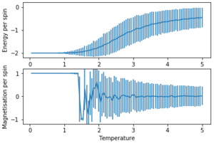
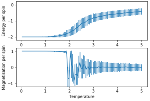

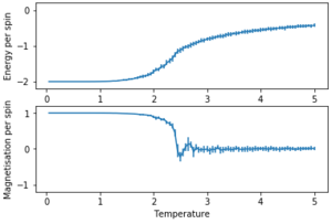
The error bars were plotted using the standard deviation.
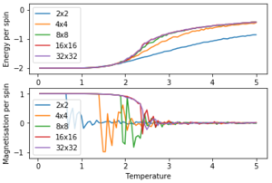
In figure 10 it can be seen that the results for a 16×16 lattice and a 32×32 lattice are similar.

With smaller lattices like a 8×8 lattice, there is not enough space to model long range fluctuations. A larger lattice like the 16×16 lattice in figure 11 can demonstrate long range fluctuations.
Section 7
From the graphs above, it is difficult to determine TC. TC could be much more easily found by plotting heat capacity against temperature. There would be a peak at T = TC.
By definition, the heat capacity
By differentiating this, a better representation can be found.
This means by plotting against T, TC can be found.

It can be seen that larger lattices produce a sharper peak.
Section 8
Data was provided of simulations which have been run for much longer. These should be more accurate.
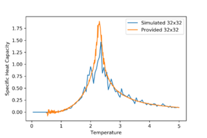
The simulated and provided data mostly fit well but the provided data has a smoother line and a sharper peak.
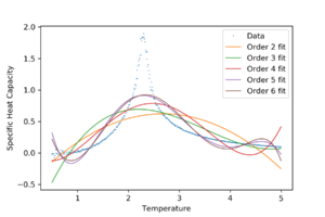
It can be seen from Figure 14 that polynomial fits over the whole temperature range do not fit very well.
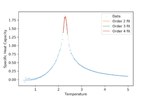
If the fit is only for data points near the peak, any polynomial above order 1 fits well. Quadratic fits will be used for following calculations. The fit was repeated for all lattice sizes.
| Lattice side length | Curie temperature |
|---|---|
| 2 | 2.54 |
| 4 | 2.45 |
| 8 | 2.35 |
| 16 | 2.32 |
| 32 | 2.30 |
Using the relation , was plotted against . The value of the y-intercept would be .
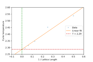
was found to be 2.29. According to literature, [1]
The agreement is quite good, only 1% off. The main sources of error are probably the large amount of fluctuations in the simulation near the Curie temperature and how a polynomial fit was used to fit a curve that should theoretically diverge.
Code
Monte Carlo simulation:
import numpy as np

class IsingLattice:


    #n_cycles = 0

    def __init__(self, n_rows, n_cols):
        #all initialisations placed in this method to always initialise properly
        #energy and magnetisation in lists to allow easier extraction of data
        self.E = []
        self.M = []
        self.n_rows = n_rows
        self.n_cols = n_cols
        self.lattice = np.random.choice([-1,1], size=(n_rows, n_cols))
        #energy and magnetisation always kept track of so that the montecarlostep method only needs to call the energy and magnetisation methods once
        self.c_energy = self.energy()
        self.c_magnetisation = self.magnetisation()
        #this cutoff works well for lattices that aren't very big
        self.cutoff = round(0.5 * (n_rows * n_cols) ** 2)
        if n_rows * n_cols > 400:
            self.cutoff = 160000

    def energy(self):
        "Return the total energy of the current lattice configuration."
        energy = -np.sum(self.lattice * np.roll(self.lattice, 1, 0) + self.lattice * np.roll(self.lattice, 1, 1))
        #energy = -sum([(self.lattice[ii, ij] * self.lattice[ii - 1, ij] + self.lattice[ii, ij] * self.lattice[ii, ij - 1]) for ii in range(self.n_rows) for ij in range(self.n_cols)])
        return energy

    def magnetisation(self):
        "Return the total magnetisation of the current lattice configuration."
        magnetisation = np.sum(self.lattice)
        #magnetisation = np.sum(c for r in self.lattice for c in r)
        return magnetisation

    def montecarlostep(self, T):
        "Performs a single Monte Carlo step"
        #the following two lines will select the coordinates of the random spin for you
        random_i = np.random.choice(range(0, self.n_rows))
        random_j = np.random.choice(range(0, self.n_cols))
        #the following line will choose a random number in the range [0,1) for you
        random_number = np.random.random()
        #changes the lattice then checks its energy
        self.lattice[random_i,random_j] *= -1
        new_energy = self.energy()
        new_magnetisation = self.magnetisation()
        #two if statements condensed into one to save time
        if random_number > np.exp((self.c_energy - new_energy) / T):
            #if the new lattice is rejected, it is reverted
            self.lattice[random_i,random_j] *= -1
        else:
            #if the new lattice is accepted, the values of energy and magnetisation are updated
            self.c_energy = new_energy
            self.c_magnetisation = new_magnetisation
        #add values of energy and magnetisation to lists
        self.E.append(self.c_energy)
        self.M.append(self.c_magnetisation)
        return [self.c_energy, self.c_magnetisation]

    def statistics(self):
        #complete this function so that it calculates the correct values for the averages of E, E*E (E2), M, M*M (M2), and returns them
        #the cutoff is applied only at this point
        return [np.mean(np.array(self.E)[self.cutoff:]), np.mean((np.array(self.E)[self.cutoff:]) ** 2), np.mean(np.array(self.M)[self.cutoff:]), np.mean((np.array(self.M)[self.cutoff:]) ** 2), len(self.E)]
Runs Monte Carlo simulation over a temperature range:
n_rows = 32
n_cols = 32
il = IsingLattice(n_rows, n_cols)
#updates the lattice without updating the energy
#this will cause the beginning of the simulation to produce erroneous but will be covered up by the cutoff point
il.lattice = np.ones((n_rows, n_cols))
spins = n_rows*n_cols
runtime = 300000
times = range(runtime)
temps = np.arange(0.05, 5.05, 0.05)
energies = []
magnetisations = []
energysq = []
magnetisationsq = []
#lists are created to keep track of the standard deviations to use for error bars
energystds = []
magnetisationstds = []
for t in temps:
    for i in times:
        if i % 10000 == 0:
            print(t, i)
        energy, magnetisation = il.montecarlostep(t)
    aveE, aveE2, aveM, aveM2, n_cycles = il.statistics()
    stdE = np.std(il.E[il.cutoff:])
    stdM = np.std(il.M[il.cutoff:])
    energies.append(aveE)
    energysq.append(aveE2)
    energystds.append(stdE)
    magnetisations.append(aveM)
    magnetisationsq.append(aveM2)
    magnetisationstds.append(stdM)
    #reset the IL object for the next cycle
    il.E = []
    il.M = []
fig = pl.figure()
enerax = fig.add_subplot(2,1,1)
enerax.set_ylabel("Energy per spin")
enerax.set_xlabel("Temperature")
enerax.set_ylim([-2.2, 0.2])
magax = fig.add_subplot(2,1,2)
magax.set_ylabel("Magnetisation per spin")
magax.set_xlabel("Temperature")
magax.set_ylim([-1.2, 1.2])
#plots including error bars
enerax.errorbar(temps, np.array(energies)/spins, yerr = np.array(energystds)/spins)
magax.errorbar(temps, np.array(magnetisations)/spins, yerr = np.array(magnetisationstds)/spins)
pl.show()
pl.savefig("32x32_2.svg")
pl.savefig("32x32_2.png")

#final data saved with extra columns for standard deviations
final_data = np.column_stack((temps, energies, energysq, energystds, magnetisations, magnetisationsq, magnetisationstds))
np.savetxt("32x32_2.dat", final_data)
Repeated for other lattice sizes (see notebook file).
Plots energy and magnetisation against temperature for all lattice sizes:
#files loaded in
d2x2 = np.loadtxt("2x2_2.dat")
d4x4 = np.loadtxt("4x4_2.dat")
d8x8 = np.loadtxt("8x8_2.dat")
d16x16 = np.loadtxt("16x16_2.dat")
d32x32 = np.loadtxt("32x32_2.dat")

#creates plot areas
fig = pl.figure()
enerax = fig.add_subplot(2,1,1)
enerax.set_ylabel("Energy per spin")
enerax.set_xlabel("Temperature")
enerax.set_ylim([-2.2, 0.2])
magax = fig.add_subplot(2,1,2)
magax.set_ylabel("Magnetisation per spin")
magax.set_xlabel("Temperature")
magax.set_ylim([-1.2, 1.2])

#plots energies
enerax.plot(d2x2[:,0], d2x2[:,1] / 4, label = "2x2")
enerax.plot(d4x4[:,0], d4x4[:,1] / 16, label = "4x4")
enerax.plot(d8x8[:,0], d8x8[:,1] / 64, label = "8x8")
enerax.plot(d16x16[:,0], d16x16[:,1] / 256, label = "16x16")
enerax.plot(d32x32[:,0], d32x32[:,1] / 1024, label = "32x32")

#plots magnetisations
magax.plot(d2x2[:,0], d2x2[:,4] / 4, label = "2x2")
magax.plot(d4x4[:,0], d4x4[:,4] / 16, label = "4x4")
magax.plot(d8x8[:,0], d8x8[:,4] / 64, label = "8x8")
magax.plot(d16x16[:,0], d16x16[:,4] / 256, label = "16x16")
magax.plot(d32x32[:,0], d32x32[:,4] / 1024, label = "32x32")

enerax.legend()
magax.legend()
pl.show()
Plots specific heat capacity against temperature for all lattice sizes:
#function defined to make plotting easier
def var_by_T2(E, E2, T):
    return (E2 - E ** 2) / (T ** 2)

pl.figure()
pl.plot(d2x2[:,0], var_by_T2(d2x2[:,1], d2x2[:,2], d2x2[:,0])/4, label = "2x2")
pl.plot(d4x4[:,0], var_by_T2(d4x4[:,1], d4x4[:,2], d4x4[:,0])/16, label = "4x4")
pl.plot(d8x8[:,0], var_by_T2(d8x8[:,1], d8x8[:,2], d8x8[:,0])/64, label = "8x8")
pl.plot(d16x16[:,0], var_by_T2(d16x16[:,1], d16x16[:,2], d16x16[:,0])/256, label = "16x16")
pl.plot(d32x32[:,0], var_by_T2(d32x32[:,1], d32x32[:,2], d32x32[:,0])/1024, label = "32x32")
pl.xlabel("Temperature")
pl.ylabel("Specific Heat Capacity")
pl.legend()
pl.savefig("C against T.png", dpi = 300)
pl.show()
Loads in the provided data files:
#provided files loaded in
c2x2 = np.loadtxt("C++_data/2x2.dat")
c4x4 = np.loadtxt("C++_data/4x4.dat")
c8x8 = np.loadtxt("C++_data/8x8.dat")
c16x16 = np.loadtxt("C++_data/16x16.dat")
c32x32 = np.loadtxt("C++_data/32x32.dat")
Plots specific head capacity against temperature for provided and simulated data:
pl.figure()
pl.plot(d32x32[:,0], var_by_T2(d32x32[:,1], d32x32[:,2], d32x32[:,0])/1024, label = "Simulated 32x32")
pl.plot(c32x32[:,0], c32x32[:,5], label = "Provided 32x32")
pl.xlabel("Temperature")
pl.ylabel("Specific Heat Capacity")
pl.legend()
pl.savefig("Comparison 32.png", dpi = 300)
pl.show()
Repeated for other lattice sizes (see notebook file).
Fits polynomials for the specific heat capacity over entire temperature range:
#creates all the polynomial fits
fit2 = np.polyfit(c32x32[:,0],c32x32[:,5],2)
fit3 = np.polyfit(c32x32[:,0],c32x32[:,5],3)
fit4 = np.polyfit(c32x32[:,0],c32x32[:,5],4)
fit5 = np.polyfit(c32x32[:,0],c32x32[:,5],5)
fit6 = np.polyfit(c32x32[:,0],c32x32[:,5],6)

#all polynomial fits plotted at once
pl.figure()
pl.plot(c32x32[:,0], c32x32[:,5], ls = "", marker = "x", ms = 1, mew = 0.5, label = "Data")
pl.plot(c32x32[:,0], np.polyval(fit2, c32x32[:,0]), lw = 1, label = "Order 2 fit")
pl.plot(c32x32[:,0], np.polyval(fit3, c32x32[:,0]), lw = 1, label = "Order 3 fit")
pl.plot(c32x32[:,0], np.polyval(fit4, c32x32[:,0]), lw = 1, label = "Order 4 fit")
pl.plot(c32x32[:,0], np.polyval(fit5, c32x32[:,0]), lw = 1, label = "Order 5 fit")
pl.plot(c32x32[:,0], np.polyval(fit6, c32x32[:,0]), lw = 1, label = "Order 6 fit")
pl.xlabel("Temperature")
pl.ylabel("Specific Heat Capacity")
pl.legend()
pl.savefig("Whole fit.png", dpi = 300)
pl.show()
Fits polynomials for the specific heat capacity over a small temperature range near the peak:
T = c32x32[:,0]
#selects values of temperature only near the peak (manually chosen)
selection = np.logical_and(T > 2.2, T < 2.4)

#creates all the polynomial fits
fit232 = np.polyfit(T[selection], c32x32[:,5][selection], 2)
fit3 = np.polyfit(T[selection], c32x32[:,5][selection], 3)
fit4 = np.polyfit(T[selection], c32x32[:,5][selection], 4)

#all polynomial fits plotted at once
pl.figure()
pl.plot(T, c32x32[:,5], ls = "", marker = "x", ms = 1, mew = 0.5, label = "Data")
pl.plot(T[selection], np.polyval(fit232, T[selection]), lw = 1, label = "Order 2 fit")
pl.plot(T[selection], np.polyval(fit3, T[selection]), lw = 1, label = "Order 3 fit")
pl.plot(T[selection], np.polyval(fit4, T[selection]), lw = 1, label = "Order 4 fit")
pl.xlabel("Temperature")
pl.ylabel("Specific Heat Capacity")
pl.legend()
pl.savefig("Cut fit.png", dpi = 300)
pl.show()
Repeated for other lattice sizes (see notebook file).
Creates a file containing curie temperatures:
#creates a file containing the curie temperatures for the five lattice sizes
np.savetxt("Curie.dat", np.column_stack(np.array([[2, 4, 8, 16, 32], [-fit22[1] / (2 * fit22[0]), -fit24[1] / (2 * fit24[0]), -fit28[1] / (2 * fit28[0]), -fit216[1] / (2 * fit216[0]), -fit232[1] / (2 * fit232[0])]])))
Plots and fits curie temperatures for different lattice sizes:
#loads curie temperatures
curiedata = np.loadtxt("Curie.dat")

#creates the straight line fit
fitcurie = np.polyfit(1 / curiedata[:,0], curiedata[:,1], 1, cov = True)

pl.figure()
pl.plot(1 / curiedata[:,0], curiedata[:,1], ls = "", marker = "x", ms = 4, mew = 0.5, label = "Data")
pl.plot([-0.2,0.7], np.polyval(fitcurie[0], [-0.2,0.7]), lw = 1, label = "Linear fit")
#plots the y axis
pl.plot([0,0],[2,3], ls = "--")
#plots a horizontal line at the y-intercept
pl.plot([-1,1],2 * [fitcurie[0][1]], ls = "--" , label = "T = 2.29")
pl.xlim([-0.1,0.6])
pl.ylim([2.25,2.6])
pl.xlabel("1 / Lattice Length")
pl.ylabel("Curie temperature")
pl.legend()
pl.savefig("Curie.png", dpi = 300)
pl.show()
Jupyter notebook containing all written code (except for simulation) including various small tests:
Yht17_CMP_Monte_Carlo_Ising.ipynb
Extras
The simulation script was modified to allow for any spin direction in 2 dimensions. Animations were made by mapping the angle of the spins onto a hsv colourmap.
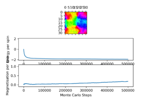
In this simulation, t = 0.1 and the lattice size is 32×32. The system has not reached equilibrium, as magnetisation is still increasing, but it is clear this is below the Curie temperature. Eventually, the domains should disappear, all the spins should align and magnetisation per spin should become close to 1, but this would be faster with a higher temperature.
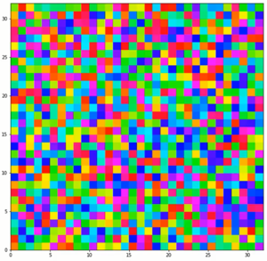

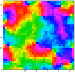
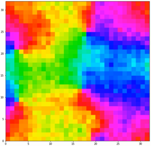
Unlike the simulations with only 2 spins states, these are able to sustain domains at low temperatures like a real ferromagnetic material such as iron. However, it still lacks interactions that are present in a real material and also lacks a dimension, so it cannot really be used effectively.
Link to full video:
Modified Monte Carlo simulation:
import numpy as np

class IsingLatticeColor:


    #n_cycles = 0

    def __init__(self, n_rows, n_cols):
        #all initialisations placed in this method to always initialise properly
        #energy and magnetisation in lists to allow easier extraction of data
        self.E = []
        self.M = []
        self.n_rows = n_rows
        self.n_cols = n_cols
        self.lattice = 2 * np.pi * np.random.random(size=(n_rows, n_cols))
        #energy and magnetisation always kept track of so that the montecarlostep method only needs to call the energy and magnetisation methods once
        self.c_energy = self.energy()
        self.c_magnetisation = self.magnetisation()
        #this cutoff works well for lattices that aren't very big
        #self.cutoff = round(0.5 * (n_rows * n_cols) ** 2)
        #if n_rows * n_cols > 400:
            #self.cutoff = 160000
        self.cutoff = 0

    def energy(self):
        "Return the total energy of the current lattice configuration."
        energy = -np.sum(np.cos(self.lattice - np.roll(self.lattice, 1, 0)) + np.cos(self.lattice - np.roll(self.lattice, 1, 1)))
        #energy = -sum([(self.lattice[ii, ij] * self.lattice[ii - 1, ij] + self.lattice[ii, ij] * self.lattice[ii, ij - 1]) for ii in range(self.n_rows) for ij in range(self.n_cols)])
        return energy

    def magnetisation(self):
        "Return the total magnetisation of the current lattice configuration."
        magnetisation = np.absolute(np.sum(np.cos(self.lattice)) + np.sum(np.sin(self.lattice)) * 1j)
        #magnetisation = np.sum(c for r in self.lattice for c in r)
        return magnetisation

    def montecarlostep(self, T):
        "Performs a single Monte Carlo step"
        #the following two lines will select the coordinates of the random spin for you
        random_i = np.random.choice(range(0, self.n_rows))
        random_j = np.random.choice(range(0, self.n_cols))
        random_a = 2 * np.pi * np.random.random()
        #the following line will choose a random number in the range [0,1) for you
        random_number = np.random.random()
        #changes the lattice then checks its energy
        self.lattice[random_i,random_j] += random_a
        new_energy = self.energy()
        new_magnetisation = self.magnetisation()
        #two if statements condensed into one to save time
        if random_number > np.exp((self.c_energy - new_energy) / T):
            #if the new lattice is rejected, it is reverted
            self.lattice[random_i,random_j] -= random_a
        else:
            #if the new lattice is accepted, the values of energy and magnetisation are updated
            self.c_energy = new_energy
            self.c_magnetisation = new_magnetisation
        self.lattice[[random_i,random_j]] = self.lattice[[random_i,random_j]] % (2 * np.pi)
        #add values of energy and magnetisation to lists
        self.E.append(self.c_energy)
        self.M.append(self.c_magnetisation)
        return [self.c_energy, self.c_magnetisation]

    def statistics(self):
        #complete this function so that it calculates the correct values for the averages of E, E*E (E2), M, M*M (M2), and returns them
        #the cutoff is applied only at this point
        return [np.mean(np.array(self.E)[self.cutoff:]), np.mean((np.array(self.E)[self.cutoff:]) ** 2), np.mean(np.array(self.M)[self.cutoff:]), np.mean((np.array(self.M)[self.cutoff:]) ** 2), len(self.E)]
Modified final frame script that also saves an animation:
import matplotlib.animation as animation

n_rows = 32
n_cols = 32
temperature = 0.1
runtime = 500001
il = IsingLatticeColor(n_rows, n_cols)
spins = n_rows*n_cols
times = range(runtime)

sfig = pl.figure(figsize = [10, 10])

E = []
M = []
L = []
for i in times:
    if i % 100 == 0:
        L.append((pl.pcolor(np.arange(0, n_rows + 1), np.arange(0, n_cols + 1), np.concatenate((np.concatenate((np.flipud(il.lattice), np.zeros((n_rows, 1))), axis = 1), np.zeros((1, n_cols + 1))), axis = 0), cmap = "hsv", vmin = 0, vmax = 2 * np.pi),))
        if i % 10000 == 0:
            print("Step", i)
    energy, magnetisation = il.montecarlostep(temperature)
    E.append(energy)
    M.append(magnetisation)
fig = pl.figure()
matax = fig.add_subplot(3,1,1)
matax.matshow(il.lattice, cmap = "hsv", vmin = 0, vmax = 2 * np.pi)
enerax = fig.add_subplot(3,1,2)
enerax.set_ylabel("Energy per spin")
enerax.set_xlabel("Monte Carlo Steps")
enerax.set_ylim([-2.1, 2.1])
magax = fig.add_subplot(3,1,3)
magax.set_ylabel("Magnetisation per spin")
magax.set_xlabel("Monte Carlo Steps")
magax.set_ylim([-0.1, 1.1])
enerax.plot(times, np.array(E)/spins)
magax.plot(times, np.array(M)/spins)
fig.savefig("animlong2ff.png", dpi = 300)


Writer = animation.writers['ffmpeg']
writer = Writer(fps=30, metadata=dict(artist='Me'), bitrate=1800)
anim = animation.ArtistAnimation(sfig, L, repeat = False)
anim.save("animlong2.mp4", writer = writer)
References
<references \>
- ↑ http://www.teori.atom.fysik.su.se/~lindroth/comp08/ising.pdf
