Investigating Ising Model Using Object Oriented Programming^[1]

Introduction

This investigation begins with the construction of a programme to model a 2D Ising lattice. The programme uses object oriented programming and Monte Carlo step function in order to model a 2D Ising lattice without having to compute all the possible system arrangements. The Ising lattice model is then tested for different lattice sizes over a range of temperatures. The total average values for energy and energy squared are stored through each temperature range computation. This prevents the need to store the energy value for each arrangement and allows for the calculation of the specific heat capacity, using the variance of the energy across each temperature range run. Five repeats were conducted for each lattice size and low order polynomial curves were fitted to the peaks of the temperature against averaged specific heat capacity plots. The maximum heat capacity was found from these fits and then the temperature at the corresponding points was taken as the Curie Temperature for each lattice size. A scaling relation was then used to calculate the Curie Temperature of an infinite lattice, thus modelling the approximate behaviour of a real ferromagnetic material.

It must be noted that all of the task titles and some formulas are copied directly from the laboratory script for clarity.^[1]

Part 1 - Introduction to the Ising model

TASK A: Show that the lowest possible energy for the Ising model is $E = - D N J$ , where $D$ is the number of dimensions and $N$ is the total number of spins. What is the multiplicity of this state? Calculate its entropy.

The interaction energy can be found using the following equation. $E = - \frac{1}{2} J \sum_{i}^{N} \sum_{j \in n e i g h b o u r s (i)} s_{i} s_{j}$

J is a constant which describes the strength of the interactions between spins. In this equation, the spins only interact with the spins adjacent to them and the equation is divided by 2 to prevent each interaction being counted twice.

The lowest energy will occur when all spins are aligned. These interactions will therefore all have a magnitude of $J$ because the product of like spins is 1 multiplied by the interaction constant $J$ . The number of interactions per spin is 2 multiplied by the number of dimensions. Therefore, the total number of interactions, when counting from the perspective of each spin, is equivalent to $2 D N$ .

Putting these observations into the original equation. $2 D N J = J \sum_{i}^{N} \sum_{j \in n e i g h b o u r s (i)} s_{i} s_{j}$ . To calculate the total energy, the factor of $- \frac{1}{2}$ must be introduced, to ensure each interaction is counted only once, and so $E_{m i n} = - D N J = - \frac{1}{2} J \sum_{i}^{N} \sum_{j \in n e i g h b o u r s (i)} s_{i} s_{j}$ .

The multiplicity of this state is equal to 2 because the spins can all be arranged parallel or all be arranged antiparallel. The entropy can be calculated using the following equation: $S = k_{b} l n Ω$ . When the multiplicity, $Ω$ , is equal to 2 then $S = k_{b} l n 2$ .

TASK B: Imagine that the system is in the lowest energy configuration. To move to a different state, one of the spins must spontaneously change direction ("flip"). What is the change in energy if this happens ( $D = 3, N = 1000$ )? How much entropy does the system gain by doing so?

The initial energy of the system can be found using $E_{m i n} = - D N J$ because all the spins are aligned. $E_{i n i t i a l} = - 3000 J$ , where J is the interaction constant. $E_{f i n a l} = - 2988 J$ because 6 interactions now have opposite spins and contribute +6J rather than -6J. Therefore $Δ E = + 12 J$ , where J is the interaction constant.

The starting entropy for the system is $S_{i n i t i a l} = k_{b} l n 2 J K^{- 1}$ because the system can only arrange itself in 2 ways. Once one spin has flipped, there is a multiplicity of 2000 because the flipped spin can occupy any of 1000 sites and this arrangement is possible when the other 999 spins are parallel or antiparallel. Therefore, $S_{f i n a l} = k_{b} l n 2000 J K^{- 1}$ and $Δ S = k_{b} (l n 2000 - l n 2) = k_{b} l n 1000 J K^{- 1}$

TASK C: Calculate the magnetisation of the 1D and 2D lattices in figure 1. What magnetisation would you expect to observe for an Ising lattice with $D = 3, N = 1000$ at absolute zero?

The magnetisation for the 1D and 2D lattices in Figure 1 of the script are +1 and +1 respectively.

For any lattice at 0 K, the maximum energy orientation would be favoured. Therefore, I would expect all the spins to be aligned either parallel or antiparallel, giving a magnetisation for the lattice in question of $\pm 1000$ .

Part 2 - Calculating the energy and magnetisation

TASK A: complete the functions energy() and magnetisation(), which should return the energy of the lattice and the total magnetisation, respectively. In the energy() function you may assume that $J = 1.0$ at all times (in fact, we are working in reduced units in which $J = k_{B}$ .

The code for both the energy and the magnetisation calculations are shown below. Both of these functions are in the IsingLattice class. The Ising Lattice being modelled here is a 2D lattice.

def energy(self):
        #Return the total energy of the current lattice configuration
        energy = 0.0
        for i in range(0,self.n_rows):
            for j in range(0,self.n_cols):
                energy = energy - (((self.lattice[i,j])*(self.lattice[((i+1)%self.n_rows),j])) + 
 ((self.lattice[i,j])*(self.lattice[i,((j+1)%self.n_cols)])))
        return energy

To calculate the energy, the interaction of all the adjacent spin interactions must be taken into account using the interaction summation formula shown in Part 1. However, rather than count the interaction for each spin with every adjacent spin, effectively counting all the interactions twice and then dividing by half as the equation does, this code only counts 2 interactions per spin. This reduces the amount of computation needed as well as the amount of code written. The code sets the energy of a lattice to 0 and then scans through every spin counting the interaction of the below spin with the current spin as well as the interaction with the spin on the right. This model is an infinite 2D lattice and so periodic boundary conditions are used. The modulus symbol '%' is used to implement these conditions. The total energy of the lattice is then returned.

 def magnetisation(self):
        #Return the total magnetisation of the current lattice configuration
        Mag = np.sum(self.lattice)
        return Mag

The magnetisation function simply executes a summation of all of the spins in the lattice and returns this total figure.

TASK B: Run the ILcheck.py script from the IPython Qt console using the command

%run ILcheck.py

Show the resulting figure.

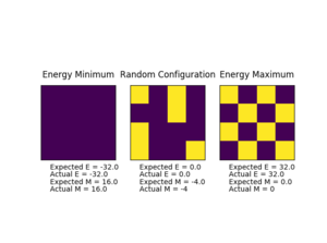
The ILcheck.py script checks the magnetisation and energy functions to ensure they are working properly, the result of one of these checks can be seen in figure 1. It outputs a 4x4 lattice with minimum energy, maximum energy and a random 4x4 lattice with the real values and the values from the tested functions. These checks will ensure that the periodic boundary conditions are maintained and that the summation part of the both functions is also giving the correct output.

Part 3 - Introduction to Monte Carlo simulation

TASK A: How many configurations are available to a system with 100 spins? To evaluate these expressions, we have to calculate the energy and magnetisation for each of these configurations, then perform the sum. Let's be very, very, generous, and say that we can analyse $1 \times 1 0^{9}$ configurations per second with our computer. How long will it take to evaluate a single value of ${⟨ M ⟩}_{T}$ ?

Each spin site can be either in the up or down position leading to the number of configurations being $2^{100}$ for 100 spin sites. To evaluate all of these configurations and find the mean magnetisation at a certain temperature, ${⟨ M ⟩}_{T}$ , with a computer that runs $1 0^{9}$ calculations per second would take $1.27 \times 1 0^{21}$ seconds. That is equivalent to $4.02 \times 1 0^{13}$ years, which is longer than the universe is thought to have existed or, in other words, too long to wait for.

TASK B: Implement a single cycle of the above algorithm in the montecarlocycle(T) function. This function should return the energy of your lattice and the magnetisation at the end of the cycle. You may assume that the energy returned by your energy() function is in units of $k_{B}$ ! Complete the statistics() function. This should return the following quantities whenever it is called: $< E >, < E^{2} >, < M >, < M^{2} >$ , and the number of Monte Carlo steps that have elapsed.

The following code is the montecarlostep function that was used during this investigation.

 def montecarlostep(self, T):
        # complete this function so that it performs a single Monte Carlo step
        initial_E = self.energy()
        #the following two lines will select the coordinates of the random spin for you
        rand_row = np.random.choice(range(0, self.n_rows))
        rand_col = np.random.choice(range(0, self.n_cols))
        self.lattice[rand_row,rand_col] = -(self.lattice[rand_row,rand_col])
        change_E = self.energy() - initial_E
        if change_E > 0:
            #the following line will choose a random number in the range [0,1) for you
            random_number = np.random.random()
            if random_number > np.exp(-change_E/T):
                self.lattice[rand_row,rand_col] = -(self.lattice[rand_row,rand_col])
        if self.n_cycles >= self.n_cycle_delay:
            self.E = self.E + self.energy()
            self.E2 = self.E2 + self.energy()**2
            self.M = self.M + self.magnetisation()
            self.M2 = self.M2 + self.magnetisation()**2
        self.n_cycles = self.n_cycles + 1
        return(self.energy(),self.magnetisation())

This function is within the class of IsingLattice and takes the temperature at which the cycles are being carried out at as an argument. A random lattice is generated to start with and a certain lattice position is selected using the numpy random.choice function, which will chose a random number from a list of coordinates. The spin at the selected lattice position is 'flipped'. The montecarlostep function will now judge using energy or probability whether this change will remain permanent. If the new arrangement is of lower energy the new lattice is accepted. If it is of higher energy than the previous lattice, then a random number between 0 and 1 is chosen and compared to the probability distribution of the energy change: $R \leq \exp {- \frac{Δ E}{k_{B} T}}$ . If the probability of the energy change is greater than the random number then the lattice is accepted, otherwise it is returned to the state it was in before the random spin flip. The states that are generated are correctly distributed because only those of low energy or high probability are likely to be selected. For example, a high energy state would have a large $Δ E$ and is therefore less likely to be selected. This step is performed many times in order to achieve a stable energy and magnetisation values of the system.

The statistics function is used to calculate the average energy, magnetism and the square of both at the end of each run. It is shown below:

 
def statistics(self):
        # complete this function so that it calculates the correct values for the averages of 
E, E*E, (E2), M, M*M (M2), and returns them
        E_av = self.E/(self.n_cycles-self.n_cycle_delay)
        E2_av = self.E2/(self.n_cycles-self.n_cycle_delay)
        M_av = self.M/(self.n_cycles-self.n_cycle_delay)
        M2_av = self.M2/(self.n_cycles-self.n_cycle_delay)
        return (E_av,E2_av,M_av,M2_av,self.n_cycles)

This function has been altered from the simple statistics function to incorporate the delay time needed for the system to equilibrate. This additional functionality will be evaluated in Part 5.

TASK C: If $T < T_{C}$ , do you expect a spontaneous magnetisation (i.e. do you expect $⟨ M ⟩ \neq 0$ )? When the state of the simulation appears to stop changing (when you have reached an equilibrium state), use the controls to export the output to PNG and attach this to your report. You should also include the output from your statistics() function.

When $T < T_{C}$ , spontaneous magnetisation is expected because the entropic contribution is less favoured at temperatures below the Curie temperature. If the entropic contribution is less favoured than the energetic contribution the spins will have a tendency to align in order to reduce the energy, therefore making the the mean magnetisation greater or less than 0. However, it is possible that two sides align with opposite spins in a metastable state, which can cause the total mean magnetisation to be close to 0.

The file ILanim was run and the results below were produced at 1 K.

After around step 500 the energy of the lattice reaches a minimum. The simulation was stopped on step 1268 and the following averaged data is given in the table below.

Figure 3 - The return of the statistics function once the simulation from figure 2 had ceased.
Averaged Quantity	Value
Energy per Spin / $k_{b}$	-1.700
Energy Squared per Spin / $(k_{b})^{2}$	3.105
Magnetisation per Spin	-0.800
Magnetisation Squared per Spin	0.733

The data is not what is expected of an equilibrated system, especially when compared to the final 700 steps on the graph. The statistics also include the first 500 unequilibrated steps and that is why the results are skewed. This is a good introductory exercise and this issue is solved later on by the improved statistics function given above.

Part 4 - Accelerating the code

It is important to find the fastest method computationally when running tests. There is usually a trade off between runtime and number of repeats and so the faster the code can run, the more data that can be collected and the more reliable the results will be.

TASK A: Use the script ILtimetrial.py to record how long your current version of IsingLattice.py takes to perform 2000 Monte Carlo steps. This will vary, depending on what else the computer happens to be doing, so perform repeats and report the error in your average!

Figure 4 shows the results of the time it takes to run 2000 Monte Carlo steps before and after the optimisation. Even though an average of around 7 seconds is slow for the initial speed, the Monte Carlo steps would have been much slower if all 4 of the adjacent spin interactions had been calculated rather than the necessary 2.

TASK B: Look at the documentation for the NumPy sum function. You should be able to modify your magnetisation() function so that it uses this to evaluate M. The energy is a little trickier. Familiarise yourself with the NumPy roll and multiply functions, and use these to replace your energy double loop (you will need to call roll and multiply twice!).

The new and improved energy function is shown below:

 def energy(self):
        #Return the total energy of the current lattice configuration
        energy = - np.sum(np.multiply(self.lattice,np.roll(self.lattice,1,0))) - np.sum(np.multiply(self.lattice,np.roll(self.lattice,1,1)))
        return energy

The double loop has been replaced by the roll function. This allows the interactions to be found by translating the same lattice one position right or down and finding the product between the translated lattice and the original. The multiply function multiplies the two values with the same lattice coordinates together producing a single lattice. A lattice is created for the right and the down translations, which, together, contain the all of the interactions. These two lattices are then summated and the total interaction is found in a single value.

TASK C: Use the script ILtimetrial.py to record how long your new version of IsingLattice.py takes to perform 2000 Monte Carlo steps. This will vary, depending on what else the computer happens to be doing, so perform repeats and report the error in your average!

The table below, figure 4, contains the data for the time it takes for the accelerated file to perform 2000 Monte Carlo steps. The accelerated code is 23 times faster and allows for longer simulations to be run during the investigation.

Figure 4 - A Table showing the improvement of the accelerated code.
Run	Time /s	Run	Times /s
Runs before Code Acceleration		Runs after Code Acceleration
1	7.401	1	0.293
2	7.063	2	0.307
3	7.044	3	0.294
4	7.007	4	0.308
5	7.045	5	0.294
6	6.997	6	0.290
7	7.015	7	0.298
8	7.041	8	0.291
9	6.986	9	0.306
10	7.003	10	0.303
Mean	7.060	Mean	0.298
Standard Deviation	0.122	Standard Deviation	0.007

The fluctuations in the performance of the code both before and after the improvement are not significant because the standard deviation is small in comparison to the values (1.73% and 2.35%). These fluctuations occur due to competing process reducing the computers processing capability.

Part 5 - The effect of temperature

TASK A: The script ILfinalframe.py runs for a given number of cycles at a given temperature, then plots a depiction of the final lattice state as well as graphs of the energy and magnetisation as a function of cycle number. This is much quicker than animating every frame! Experiment with different temperature and lattice sizes. How many cycles are typically needed for the system to go from its random starting position to the equilibrium state? Modify your statistics() and montecarlostep() functions so that the first N cycles of the simulation are ignored when calculating the averages. You should state in your report what period you chose to ignore, and include graphs from ILfinalframe.py to illustrate your motivation in choosing this figure.

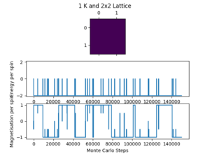
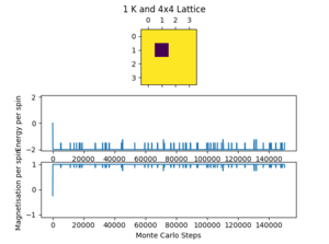
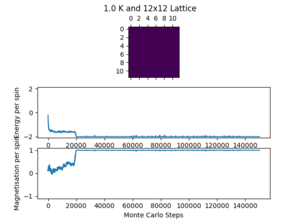
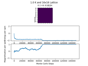
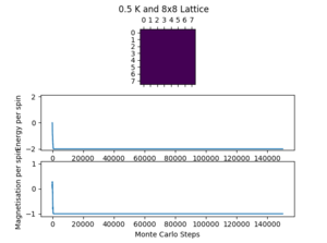
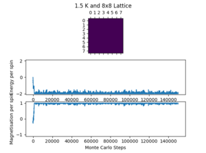
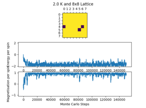
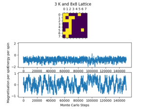
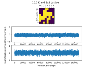
Figures 5 and 6 below show how long each system takes to equilibrate with lattice size and temperature respectively. The number of cycles taken to equilibrate is an approximation from the data available (the pictures included in the figures are a few of many and the results were determined from this wider range of results). There can be quite large fluctuations in equilibrium time due to the randomness involved with the Monte Carlo step and the possibility of the lattice reaching a metastable state.

Figure 5 - Shows the effect of lattice size on the number of cycles taken to equilibrate at 1 K
Lattice Size	Approximation for Number of Cycles to Equilibrate	Cycle Delay Imposed
2x2	100	1,000
4x4	200	2,000
8x8	1,000	10,000
12x12	25,000	N/A
16x16	50,000	50,000
18x18	100,000	N/A
32x32	150,000	150,000

The table above shows a sharp increase in the number of cycles needed to equilibrate when the lattice size increases. This was expected before the simulation was run because the more lattice positions there are, the less likely each position is chosen in a Monte Carlo step. Also, the metastable state of a larger lattice is more stable because a single spin change has relatively less of an effect on the whole lattice.

Figure 6 - Shows the effect of temperature on the number of cycles taken to equilibrate for an 8x8 lattice
Temperature /K	Approximation for Number of Cycles to Equilibrate	Example PNG
0.5	500
1.0	1,000
1.5	1,000
2.0	2,000
3.0	Begins in equilibrium
10.0	Begins in equilibrium

Figure 6 shows the change in equilibration time with temperature. There is a small apparent increase in equilibration time from 0.5 K to 2 K, but it is difficult to conclude so with confidence. As the temperature increases further, the Curie Temperature is surpassed, and the lattice has begins and continues in random equilibrium. The equilibration time at 3 K and 10 K is therefore 0 cycles. From these results it is also possible to make a tentative conclusion that the Curie Temperature of the 8x8 lattice lies between 2 K and 3 K.

When results are recorded later in the investigation it is necessary to remove the effect of the random lattice produced at the start. This is because the random lattice does not represent the actual lattice, it is just a starting point and these initial results may skew the overall value. Therefore, a cycle delay is implemented to reduce this. The values for the cycles delay imposed (figure 5) may seem very safe for the 2x2, 4x4 and 8x8, but with the short equilibration times, there is relatively very little loss at increasing the cycle delay. For the 16x16 and, especially, the 32x32 lattice there was a trade off between computation time and accuracy (the delay of 150,000 for the 32x32 lattice and 150,000 further cycles took 40 minutes to run over the temperature range, with a total of around 4 hours for all 5 repeats). The cycle delay chosen for both is reasonable but there is a risk that a metastable state could remain into the cycles that are counted. To combat this, the resulting output graphs from ILtemperaturerange.py were used as feedback and checked to ensure that one of the points had not been affected by this problem.

A new class variable n_cycle_delay was created to implement the cycle delay. The modified statistics function can be seen in Part 3B and the edited part of the montecarlostep function can be seen below:

 
(self.lattice[rand_row,rand_col])
        if self.n_cycles >= self.n_cycle_delay:
            self.E = self.E + self.energy()
            self.E2 = self.E2 + self.energy()**2
            self.M = self.M + self.magnetisation()
            self.M2 = self.M2 + self.magnetisation()**2
        self.n_cycles = self.n_cycles + 1
        return(self.energy(),self.magnetisation())

The cycle delay prevents the collection of data until the number of cycles is greater than the delay. The statistics functions accounts for this and only divides by the number of cycles counted.

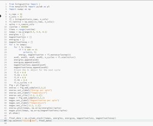
TASK B: Use ILtemperaturerange.py to plot the average energy and magnetisation for each temperature, with error bars, for an $8 \times 8$ lattice. Use your intuition and results from the script ILfinalframe.py to estimate how many cycles each simulation should be. The temperature range 0.25 to 5.0 is sufficient. Use as many temperature points as you feel necessary to illustrate the trend, but do not use a temperature spacing larger than 0.5. The NumPy function savetxt() stores your array of output data on disk — you will need it later. Save the file as 8x8.dat so that you know which lattice size it came from.

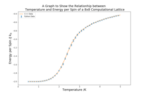
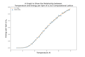
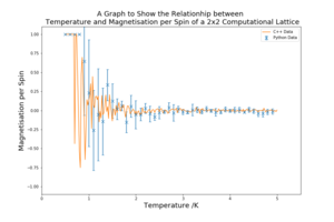
The script ILtemperaturerange.py was used to find the relationship between energy and temperature and magnetisation and temperature. The lattice tested for this task is 8x8. The temperatures tested were in the range 0.5 K to 5 K and taken every 0.1 K. The number of Monte Carlo steps run at each temperature was 100,000, with the first 10,000 not being used to collect. The reasons for this decision are in Part 5 Task A. There were 5 repeats of the ILtemperaturerange.py runs in order to achieve more reliable results and to find the standard deviation of the repeats for each temperature point. The data is plotted against the C++ data provided for reference.

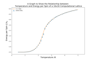
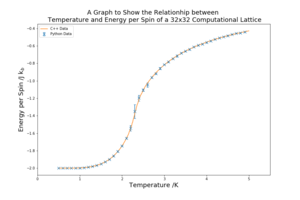
The temperature against energy plot in figure 7 shows an increase in energy per spin of the system with temperature. As temperature increases the entropic component of the system becomes larger until it dominates and the system is at random dynamic equilibrium. At low temperatures the energy per spinis very close to -2 $k_{b} J$ because all the spins are aligned. In the area of transition between entropically driven equilibrium and energetically driven equilibrium there is a higher standard deviation of the results, represented by the larger error bars. This is also an area of high importance as the Curie temperature is located in this region. Figure 9 shows the adjusted code of ILtemperaturerange.py to receive results for this lattice size.

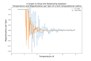
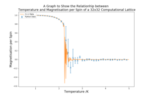
Figure 8 shows the effect of temperature on magnetisation per spin. The magnetisation per spin is at +1 at low temperatures because it is more favourable to have the spins aligned. As the temperature increases the entropic component becomes larger and the system prefers a more random orientation of spins and the magnetisation per spin becomes close to zero. In the region of the graph when magnetisation per spin changes from +1 to 0, the standards deviation for the points is the largest and the magnetisation per spin is much more volatile. The collected data is very similar to the C++ data provided.

Part 6 - The effect of system size

TASK A: Repeat the final task of the previous section for the following lattice sizes: 2x2, 4x4, 8x8, 16x16, 32x32. Make sure that you name each datafile that your produce after the corresponding lattice size! Write a Python script to make a plot showing the energy per spin versus temperature for each of your lattice sizes. Repeat this for the magnetisation. As before, use the plot controls to save your a PNG image of your plot and attach this to the report. How big a lattice do you think is big enough to capture the long range fluctuations?

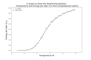
For each of the lattice sizes and their respective plots, in figure 10 below, the temperature range is 0.5 K to 5 K with a spacing of 0.1 K. The range covers both the region above and below the Curie temperature comprehensively. The smaller the spacing between the temperatures the better, as more results are achieved, but, especially for the larger lattices, the tighter the spacing the longer the computation. The spacing of 0.1 K provides enough points in each region of the graph to make significantly accurate plots. 5 repeats were conducted for each lattice size, allowing for random error to be reduced and a meaningful standard deviation to be found. The C++ data provided is also plotted against the curves for reference.

Figure 10 - Compilation of all the temperature vs energy per spin and temperature vs magnetisation per spin plots for the 2x2, 4x4, 8x8, 16x16 and 32x32 lattices.
Lattice Size	Total Number of Cycles	Number of Delayed Cycles
2x2	10,000	1,000
4x4	20,000	2,000
8x8	100,000	10,000
16x16	150,000	50,000
32x32	150,000	150,000

The graphs in figure 10 show a sharpening of the curves for both magnetisation and energy as the lattice size increases. In the temperature vs energy per spin plots the transition region in the centre of the graph becomes shorter. The entropically dominated and energetically dominated regions become clearer and more consistent. In the temperature vs magnetisation per spin plots a similar effect is seen as the lattice size is increased, the region where the spins are aligned is maintained at higher temperatures and the transition region is shortened. In all plots the standard deviation is the highest in the transition region. The collected data resembles the C++ in all of the plots.

Looking at the magnetisation graphs, the long range fluctuations decrease the larger the lattice size. The 2x2 lattice graph contains several fluctuations, whereas the 32x32 lattice graph contains only a few around the transition from +1 to 0. However, the 32x32 lattice does not contain a smooth curve in the transition region and a larger lattice size of potentially 64x64, or even more, would minimise the fluctuations in this region to a smooth curve.

Part 7 - Determining the heat capacity

TASK A^[2]: By definition,

$C = \frac{\partial ⟨ E ⟩}{\partial T}$

From this, show that

$C = \frac{V a r [E]}{k_{B} T^{2}}$

(Where $V a r [E]$ is the variance in $E$ .)

The average energy of a canonical ensemble is:

 $⟨ E ⟩ = \sum_{n} p (n) E_{n} = \sum_{n} \frac{E_{n} e^{- β E_{n}}}{Z} E q u a t i o n 1$

This can be expressed more simply with respect to the partition function as:

 $⟨ E ⟩ = - \frac{\partial}{\partial β} l o g Z E q u a t i o n 2$

The spread of the energies about the mean is shown by the variance. The variance can be found if the mean of the energy and the mean of the energy squared is known, using the sum of squares relation rather than the usual summation of every result. This is shown as:

 $V a r [E] = Δ E^{2} = ⟨ (E - ⟨ E ⟩)^{2} ⟩ = ⟨ E^{2} ⟩ - {⟨ E ⟩}^{2} E q u a t i o n 3$

Written once again in terms of the partition function:

 $Δ E^{2} = \frac{\partial^{2}}{\partial β^{2}} l o g Z = - \frac{\partial ⟨ E ⟩}{\partial β} E q u a t i o n 4$

This can be related to the specific heat capacity of the canonical ensemble, which represents the change in mean energy with respect to temperature at a constant volume:

 $C_{v} = (\frac{\partial ⟨ E ⟩}{\partial T})_{v} E q u a t i o n 5$

With $V a r [E] = Δ E^{2}$ , the relation of $β = 1 / k_{b} T$ allows equations 4 and 5 to be combined to form:

 $C = \frac{V a r [E]}{k_{B} T^{2}} E q u a t i o n 6$

TASK B: Write a Python script to make a plot showing the heat capacity versus temperature for each of your lattice sizes from the previous section. You may need to do some research to recall the connection between the variance of a variable, $V a r [X]$ , the mean of its square $⟨ X^{2} ⟩$ , and its squared mean ${⟨ X ⟩}^{2}$ . You may find that the data around the peak is very noisy — this is normal, and is a result of being in the critical region. As before, use the plot controls to save your a PNG image of your plot and attach this to the report.

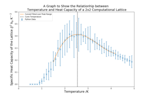
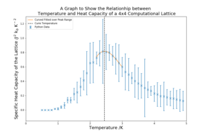
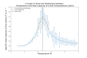
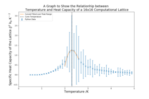
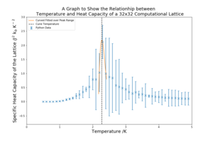
For each of the lattice sizes and their respective temperature vs heat capacity plots, in figure 11 below, the temperature range is 0.5 K to 5 K with a spacing of 0.1 K. 5 repeats were conducted for each lattice size, allowing for random error to be reduced and a meaningful standard deviation to be found. The C++ data provided is also plotted against the curves for reference. The heat capacity is calculated using equation 6 in Part 7B. The units are carried through from equation 6, having used the Boltzmann factor in the previous energy values.

Figure 11 - Temperature vs Heat Capacity plots for all the lattices sizes.
Lattice Size	Heat Capacity Plot
2x2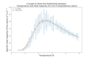
4x4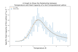
8x8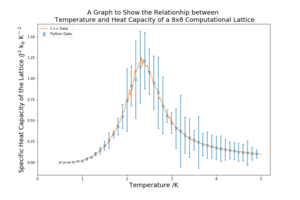
16x16
32x32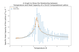

As the lattice size increases the peak becomes sharper and more defined. The peaked region in the middle also has higher standard deviation that the other regions of the graph. This critical region contains the Curie Temperature, the temperature at which the permanent magnetic properties are lost. The heat capacity at the Curie temperature should, in theory, be infinity because it marks a transition. However, as the lattice sizes are small, this region is broadened and a does not diverge, the sharpening of the peaks is an indication that an infinite lattice could achieve this divergence.

The standard deviations for a lot of graph are very high, which will contribute to the overall error of the investigation.

Part 8 - Locating the Curie temperature

TASK A: A C++ program has been used to run some much longer simulations than would be possible on the college computers in Python. You can view its source code here if you are interested. Each file contains six columns: $T, E, E^{2}, M, M^{2}, C$ (the final five quantities are per spin), and you can read them with the NumPy loadtxt function as before. For each lattice size, plot the C++ data against your data. For one lattice size, save a PNG of this comparison and add it to your report — add a legend to the graph to label which is which. To do this, you will need to pass the label="..." keyword to the plot function, then call the legend() function of the axis object (documentation here).

The graphs requested by this are in figure 11 in Part 7B. For lattice sizes 2x2, 4x4 and 8x8 the C++ data is very similar to that of the data acquired using object orientated programming in this investigation. For the 16x16 and 32x32 lattice sizes all parts of the graph except for the peak are similar. For the 16x16 lattice the C++ data has a higher peak and in the 32x32 lattice the C++ data has a lower peak. This is not particularly concerning as the C++ data is well within one standard deviation of the points around the peak but the difference in peak size will make a difference when fitting a curve to the peak later in the investigation.

TASK B: write a script to read the data from a particular file, and plot C vs T, as well as a fitted polynomial. Try changing the degree of the polynomial to improve the fit — in general, it might be difficult to get a good fit! Attach a PNG of an example fit to your report.

To begin with low order polynomial fits were attempted in order to achieve a good fit from the curves. Figure 12 shows the result of a third order fit and the result is a horrendous fit to the data. Through testing many different polynomial orders better fits were then found as shown in figure 13 and 14, which use a 20th and 28th order fit respectively.

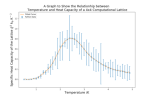
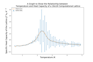
Even though the orders of the good fits may seem slightly ridiculous, the modelling of the fits at the peak especially is smooth and the fits include all of the data points. However, the peaks of the curves are not of such high orders and so these fits, although they look satisfactory, may misrepresent the peaks. Therefore, the peaks should be modelled using lower order polynomials. This is executed in the next task.

TASK C: Modify your script from the previous section. You should still plot the whole temperature range, but fit the polynomial only to the peak of the heat capacity! You should find it easier to get a good fit when restricted to this region.

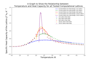
The fits of low order polynomials (2 or 3) are made across the peak region of graphs. These can vary based on which points are chosen to be included and what order the polynomial is selected as. The high standard deviation in this region also makes it difficult to have significant confidence in the fits. The fits for all of the lattice sizes' peaks are shown in figure 15 below. The figure also contains a graph with all of the fits plotted together.

Figure 15 - Shows all of the peak fits for the Temperature vs Heat Capacity data for all lattices and the temperature range the fits were plotted over
Lattice Size	Temperature Range Used in Fitting /K	Order of Polynomial Used in Fitting
2x2	1.5 - 4.2	3
4x4	2.2 - 3.0	3
8x8	2.0 - 2.8	3
16x16	2.0 - 2.6	3
32x32	2.1 - 2.5	3
All lattices	N/A	N/A

The plots in figure 15 contain the low order polynomial fits to the peak value of the curve. The fits are much better than in Part 8B and represent the peak values of the curve with a reasonable order of fit. However, as the lattice size increases and the curve becomes sharper, the fewer points either side of the peak it is possible to take and maintain a good fit. The fewer points that are used the less reliable the fit and it is important to note that the fit is made to points with very high standard deviations. The graph with all of the temperature vs heat capacity plots is a good illustration of the graph maximums increasing in magnitude and decreasing in temperature value as the lattice size increases. The Curie Temperature at the peak of the fits is marked onto each of the graphs in preparation for Part 8D.

TASK D: find the temperature at which the maximum in C occurs for each datafile that you were given. Make a text file containing two columns: the lattice side length (2,4,8, etc.), and the temperature at which C is a maximum. This is your estimate of $T_{C}$ for that side length. Make a plot that uses the scaling relation given above to determine $T_{C, \infty}$ . By doing a little research online, you should be able to find the theoretical exact Curie temperature for the infinite 2D Ising lattice. How does your value compare to this? Are you surprised by how good/bad the agreement is? Attach a PNG of this final graph to your report, and discuss briefly what you think the major sources of error are in your estimate.

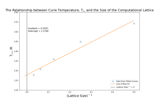
The $T_{c}$ was found for all of the lattice sizes using the fitted curves from Part 8C. Figure 16 shows the plot of the inverse of lattice size against $T_{c}$ in accordance with the scaling relation: $T_{C, L} = \frac{A}{L} + T_{C, \infty}$ . The intercept is at the $T_{c}$ where the inverse of of the lattice size is zero, which is an infinite lattice.

The intercept or $T_{C, \infty}$ is equal to 2.2790, which has only a 0.441 % difference with the literature value of 2.269.^[3] This agreement is surprisingly good considering the high standard deviations at the peak points and the variability of the peak fits depending on the temperature range taken. I think these two issues aforementioned are the main sources of error. The standard deviation is very high in the peaks of the temperature vs heat capacity graphs because the error in both energy and energy squared contributes twice to the variance. The critical region also contains the highest initial error, which is amplified at the peak heat capacity. The fitting of the graphs is also a large source of error. It is difficult to balance including more points or getting a more visually accurate fit. Depending on the fit chosen the overall answer will change. These errors can be reduced by conducting more repeats and evaluating a great number of lattice sizes. A smaller temperature spacing could also have been used to more reliably find the specific heat capacity peak maximum.

Conclusion

The investigation yielded values very close to the literature value, considering the number of lattice sizes and repeats conducted, to get a result with less than 1 % difference to literature value constitutes a successful investigation.The use of object programming and data abstraction has allowed good results to be found in a comparatively short period of time. However, with the high error in the heat capacity data and the difficulties in fitting the polynomial curves, it is not possible to have complete confidence in the investigation's findings.

Additional Material

Extra Graph

For Part 8D, an additional graph was plotted in order to investigate the scaling relation, also in Part 8D. The scaling relation was multiplied by the lattice size to produce the following equation and graph:

 $T_{C, L} L = A + T_{C, \infty} L$

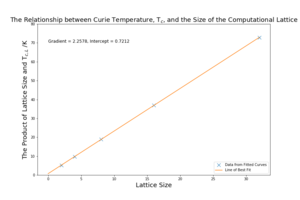
The gradient in figure 17, which is equivalent to $T_{C, L}$ , is 2.258, which has a percentage difference of 0.485 % with the literature value of 2.269. This graph looks to have a more appropriate fit, is not affected by the constant A along any of the gradient and does not require the extrapolation of data. However, the lattice size is used as part of the dependent and independent variable, which is not favourable.

Analytical Code

Two of the most favoured analytical functions will be included here. The ultimate aim of the analysis was to create functions that receive but a few arguments to evaluate the entirety of the data with little effort.

def graph_maker_C_with_fit_ranged(input_file_list, lattice_size, 
output_file,order,T_max,T_min,y1,y2):
    Temperature,E,E2,M,M2 = average_file_killa
(input_file_list,lattice_size)
    Temp_range,fitted_c = poly_fitter_ranged
(Temperature,E,E2,order,lattice_size,T_max,T_min)
    figure(figsize=[12,8])
    T2 = np.power(Temperature,2)
    mu_sq = np.power(E,2)*(lattice_size**2)
    Var = np.subtract(E2,mu_sq)
    errorbar(Temperature,(Var/T2),yerr=std_file_killa_C(input_file_list,lattice_size)
,label='Python Data', marker= 'x', linestyle= ' ', ms=8, capsize=3)
    plot(Temp_range,fitted_c, label='Curved Fitted over Peak Range')
    Max_t = Temp_range[fitted_c==np.max(fitted_c)]
    plot(linspace(Max_t,Max_t,1000),linspace(-1,10,1000), 
label='Curie Temperature',linestyle='--',color='black')
    title('A Graph to Show the Relationhip between \n Temperature and Heat Capacity of a ' + 
str(lattice_size) + 'x' + str(lattice_size) + ' Computational Lattice', fontsize=18)
    xlabel('Temperature /K', fontsize=18)
    legend(loc='upper left')
    ylim(y1,y2)
    xlim(0,5)
    ylabel('Specific Heat Capacity of the Lattice 
/$J^2$ k$_{b}$ K$^-$$^2$', fontsize=18)
    savefig( 'jh6215_' + output_file)
    show()
    return

This code takes a list of 5 files (packed using a different function), one for each temperature range repeat, the lattice size, the name of the final image file and some graphical numbers. From these inputs only, the graphs with curves fitted across the peak region, as seen in Part 8C are plotted in one line of code including this function.

def std_file_collector(file_list,lattice_size):
    loaded_list = []
    E_std = []
    E_Var = []
    for file1 in file_list:
        loaded_list= loaded_list + [loadtxt(file1)]
    n_temps = len(loaded_list[1])
    for row in range(0,n_temps):
        e = []
        for file1 in loaded_list:
            e = e + [file1[row][1]/(lattice_size**2)]
        E_std = E_std + [np.std(e)]
    return E_std

This function takes only the file list of the 5 temperature range repeat files and the lattice size. It outputs a list of the standard deviations of the energy without depending on any previous working.

References

↑ ^1.0 ^1.1 Third year CMP compulsory experiment Laboratory Script, 2017, https://wiki.ch.ic.ac.uk/wiki/index.php?title=Third_year_CMP_compulsory_experiment
↑ D. Tong, Statistical Physics, 2011, 20, http://www.damtp.cam.ac.uk/user/tong/statphys/sp.pdf
↑ J. Kotze, Introduction to Monte Carlo methods for an Ising Model of a Ferromagnet, 2008, 22, https://arxiv.org/pdf/0803.0217.pdf

[:0-1] 1.0 ^1.1 Third year CMP compulsory experiment Laboratory Script, 2017, https://wiki.ch.ic.ac.uk/wiki/index.php?title=Third_year_CMP_compulsory_experiment

[2] D. Tong, Statistical Physics, 2011, 20, http://www.damtp.cam.ac.uk/user/tong/statphys/sp.pdf

[3] J. Kotze, Introduction to Monte Carlo methods for an Ising Model of a Ferromagnet, 2008, 22, https://arxiv.org/pdf/0803.0217.pdf

[1]

[2]

[3]

Investigating Ising Model Using Object Oriented Programming[1]