Rep:CMP3:IM915
Introduction to the Ising Model
The Model
The Ising model is a physical model used to describe and understand ferromagnets- materials where there is preferential alignment of magnetic dipoles along certain directions and therefore an overall magnetic moment. While all spins aligned is more energetically favourable, this is the minimum entropy state, and the balance between entropy maximisation and energy minimisation leads to a phase transition.
In the Ising model, a collection of spins is considered arranged on a lattice (a line in 1D, a grid in 2D, a cuboid in 3D). When no magnetic field is applied, the only contribution to energy is from the interaction of adjacent spins. Periodic boundary conditions are applied.
Total interaction energy is defined by the equation:
Where is a constant which controls the strength of interaction and indicates adjacent spins.
TASK: Show that the lowest possible energy for the Ising model is , where is the number of dimensions and N is the total number of spins. What is the multiplicity of this state? Calculate its entropy.
The lowest energy state for the Ising model (with no applied field) will be all spins aligned (either all up or all down).
Therefore, using the equation for total energy:
Total energy .
As all spins are aligned,
The number of neighbours is related to dimensionality- in 1D each spin has 2 neighbours, in 2D each spin has 4, and in 3D each spin has 6 - i.e. there are 2D neighbours.
Total energy = .
Total energy .
The multiplicity of this state is 2, as there are two degenerate configurations with all spins aligned (all spins = +1, and all spins = -1).
Entropy is calculated from multiplicity using the Boltzmann's Entropy Equation where W is multiplicity and kb is the Boltzmann Constant:
Phase Transitions
Provided a lattice of 2 or more dimensions is used, the Ising model displays a phase transition. The temperature controls the balance between energetics (favouring lowest energy configuration) and entropy (favouring the configuration with the maximum number of degenerate states).
TASK: Imagine that the system is in the lowest energy configuration. To move to a different state, one of the spins must spontaneously change direction ("flip"). What is the change in energy if this happens (D=3,\ N=1000)? How much entropy does the system gain by doing so?
When a single spin is flipped, all its interactions with its neighbours are now unfavourable rather than favourable. Therefore for this one particular spin, as .
Therefore,
Total energy =
Therefore, the total energy change of the system is equal to , which is equal to 6J in this case (D=3).
The entropy change of the system can be calculated by considering the change in number of configurations. The number of configurations of a system with 1000 spins where a single spin is flipped is 2000 (1000 with the single spin = +1, and 1000 with the single spin = -1).
So the entropy of the new system is equal to .
Entropy change = .
TASK: Calculate the magnetisation of the 1D and 2D lattices in figure 1. What magnetisation would you expect to observe for an Ising lattice with D = 3,\ N=1000 at absolute zero?
Total magnetisation of the system .

The magnetisation of the 1D lattice shown above is +1, and the 2D lattice also has a magnetisation of +1.
At absolute zero, an Ising lattice will have all spins aligned (all either +1 or all either -1). The magnetisation I would expect for an Ising lattice with is
Calculating the energy and magnetisation
Modifying the files
An IsingLattice class is defined, which contains the function __init__, and the empty functions energy(), magnetisation() and statistics().
IsingLattice(x,x) creates an IsingLattice object with x rows and x columns, with random spins.
TASK: complete the functions energy() and magnetisation(), which should return the energy of the lattice and the total magnetisation, respectively. In the energy() function you may assume that J=1.0 at all times (in fact, we are working in reduced units in which J=k_B, but there will be more information about this in later sections). Do not worry about the efficiency of the code at the moment — we will address the speed in a later part of the experiment.
The initially created functions for energy() and magnetisation are given below:
Energy
def energy(self):
"Return the total energy of the current lattice configuration. Assumes J = 1 at all times"
    for i in range(0,self.n_rows):
        for j in range(0,self.n_cols):
            pos_0 = self.lattice[i,j]
            pos_1 = self.lattice[i-1,j]
            pos_2 = self.lattice[i,j-1]
            pos_3 = self.lattice[i,(j+1)%self.n_cols]
            pos_4 = self.lattice[(i+1)%self.n_rows,j]
            energy_sum += pos_0*pos_1 + pos_0*pos_2 + pos_0*pos_3 + pos_0*pos_4
            energy = -energy_sum/2
Magnetisation
def magnetisation(self):
"Return the total magnetisation of the current lattice configuration."
    magnetisation = np.sum(self.lattice)
Testing the files
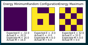
The provided ILcheck.py script creates three IsingLattice objects and returns both the true energies and magnetisation, along with those generated by the previously written energy() and magnetisation() functions.
TASK: Run the ILcheck.py script from the IPython Qt console using the command
%run ILcheck.py
The displayed window has a series of control buttons in the bottom left, one of which will allow you to export the figure as a PNG image. Save an image of the ILcheck.py output, and include it in your report.
The check function shows that my energy and magnetisation functions work, as the expected and actual energy are equal.
Introduction to Monte Carlo simulation
Average Energy and Magnetisation
The statistical mechanics equations for average energy and magnetism, as functions of temperature, are shown below.
TASK: How many configurations are available to a system with 100 spins? To evaluate these expressions, we have to calculate the energy and magnetisation for each of these configurations, then perform the sum. Let's be very, very, generous, and say that we can analyse configurations per second with our computer. How long will it take to evaluate a single value of ?
A system of 100 spins has a total of configurations. (Each spin has two possible orientations, and number of spins = 100). This is equal to configurations. If configurations can be analysed per second, to analyse every configuration will take seconds.
seconds
This is equal to years, i.e. 4 thousand billion years.
Importance Sampling
In order to allow simulations to be run within reasonable time-frames, a smarter approach to analysing average energy and magnetism is required. The Bolzmann factor, , is very small for the majority of configurations and these can therefore be ignored. By only considering the states with a relatively large Boltzmann factor, a simulation can be run within a reasonable time-frame.
The Monte Carlo Method allows us to do this, by generating states randomly from the Boltzmann probability distribution. The algorithm is as follows.
- 1. Start from a given configuration of spins with energy
- 2. Choose a single spin at random and flip it, to give configuration
- 3. Calculate the new energy,
- 4. Calculate the energy difference,
- 4.1 If then the spin flipping decreased the energy and the new configuration is accepted. Set and . Go to step 5
- 4.2 If , spin flipping increased the energy and so the probability must be considered. The probability for the transition to occur is . To ensure we select with the correct probability, we use the procedure;
- a) Choose a random number R in the interval [0,1)
- b) If , we accept the new configuration, set and and go to step 5.
- c) If If , we reject the new configuration, leave and unchanged and go to step 5
- 5. Update running averages of energy and magnetism
- 6. Monte Carlo cycle complete. Return to Step 2
Modifying IsingLattice.py
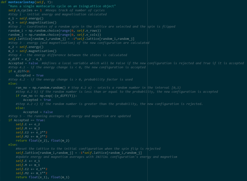
TASK: Implement a single cycle of the above algorithm in the montecarlocycle(T) function. This function should return the energy of your lattice and the magnetisation at the end of the cycle. You may assume that the energy returned by your energy() function is in units of k_B! Complete the statistics() function. This should return the following quantities whenever it is called: <E>, <E^2>, <M>, <M^2>, and the number of Monte Carlo steps that have elapsed.

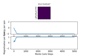
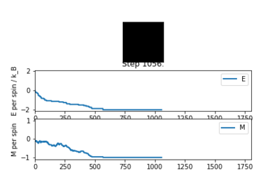
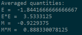
TASK: If , do you expect a spontaneous magnetisation (i.e. do you expect ? When the state of the simulation appears to stop changing (when you have reached an equilibrium state), use the controls to export the output to PNG and attach this to your report. You should also include the output from your statistics() function.
If , then spontaneous magnetisation is expected. Tc is the curie temperature, above which materials lose their permanent magnetic properties. At temperatures below Tc the material will still have permanent magnetism. At temperatures above Tc the temperature is high enough that the increase in entropy by having random spin alignment is large enough to compensate for the fact random alignment is less energetically favorable.
A simulation was run with an 8x8 lattice at T = 1 (below the Curie Temperature).
Accelerating the Code
TASK: Use the script ILtimetrial.py to record how long your current version of IsingLattice.py takes to perform 2000 Monte Carlo steps. This will vary, depending on what else the computer happens to be doing, so perform repeats and report the error in your average!
ILTimetrial.py was run 20 times and the times taken recorded. The average time to perform 2000 Monte Carlo steps was 4.82 seconds. Standard deviation was equal to 0.44 seconds, and therefore the standard error of the mean (SEM) was equal to 0.098 seconds.
TASK: Look at the documentation for the NumPy sum function. You should be able to modify your magnetisation() function so that it uses this to evaluate M. The energy is a little trickier. Familiarise yourself with the NumPy roll and multiply functions, and use these to replace your energy double loop (you will need to call roll and multiply twice!).
The sum function was already being used to calculate magnestisation() (code repeated again below) from the initial draft of the function, and so this function could not be improved.
magnetisation = np.sum(self.lattice)
The energy function however was inefficient, and was improved using roll and multiply. The modified energy function is shown below.

TASK: Use the script ILtimetrial.py to record how long your new version of IsingLattice.py takes to perform 2000 Monte Carlo steps. This will vary, depending on what else the computer happens to be doing, so perform repeats and report the error in your average!
ILtimetrial.py was run 20 times again on the modified code, and the times taken were recorded. The average time to perform 2000 Monte Carlo steps was 0.31 seconds, over 10 times faster than the initial code. Standard deviation was equal to 0.055 seconds, and therefore the standard error of the mean (SEM) was equal to 0.012 seconds.
The effect of temperature
When starting from a random configuration (as we do here) it takes a certain amount of Monte Carlo cycles to reach the equilibrium state, during which the energy rapidly drops and magnetisation rapidly changes. To calculate accurate averages of the system, these first steps should be disregarded.
TASK: The script ILfinalframe.py runs for a given number of cycles at a given temperature, then plots a depiction of the final lattice state as well as graphs of the energy and magnetisation as a function of cycle number. This is much quicker than animating every frame! Experiment with different temperature and lattice sizes. How many cycles are typically needed for the system to go from its random starting position to the equilibrium state? Modify your statistics() and montecarlostep() functions so that the first N cycles of the simulation are ignored when calculating the averages. You should state in your report what period you chose to ignore, and include graphs from ILfinalframe.py to illustrate your motivation in choosing this figure.
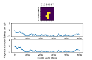
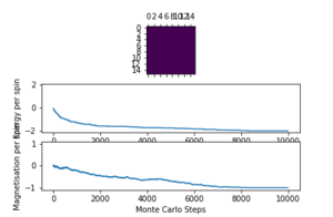
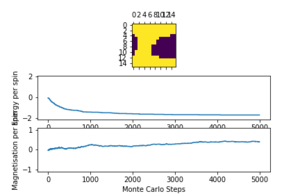
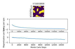
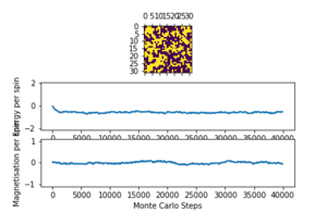
The number of steps required for the system to reach equilibrium varies with lattice size and temperature. At smaller lattice sizes, the system reaches equilibrium much faster, which is always the lowest energy configuration. However at higher lattice sizes the system often gets stuck in meta-stable states where the system is not in the lowest energy configuration but is stuck in a local energy minimum, which is stable enough that a single spin flip is not enough to escape the well. At higher temperatures, the time taken to equilibrate is longer, and at high enough temperatures (above the curie temperature) the system equilibrates at points away from the minimum energy energy configuration, and new magnetisation decreases. Some images are shown below that demonstrate this.
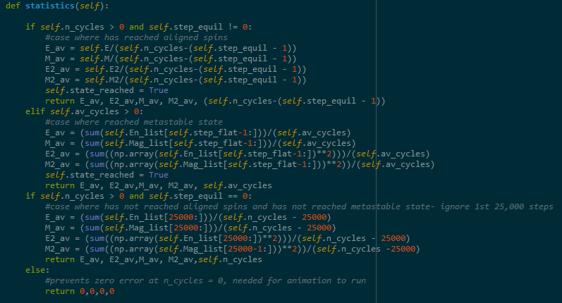
Instead of choosing an arbitrary figure for number of points to discard, a method was added to the code to locate the point of equilibrium and reject all points before.
For points where the lattice reaches the fully aligned state (lowest energy), this was easy to implement as the point when the fully aligned state is reached can be used as the point of equilibration. The code is shown below.

For points where the lattice equilibrates but not at a fully aligned state, a different method was needed. A running list of energies was generated, and two points 10,000 steps apart were compared. If the difference in energy was less than a certain value (determined by experimentation), the system was supposed to have equilibrated.

The statistics function was updated to return the correct average for these cases, and an extra case was added where the system never equilibrated according to either method above- the first 25,000 steps were ignored, as all systems were equilibrated long before this point.
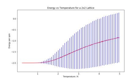
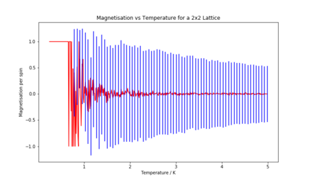
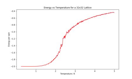
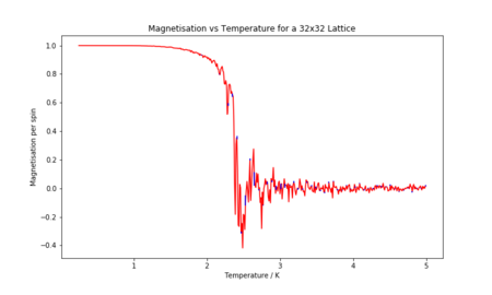
TASK: Use ILtemperaturerange.py to plot the average energy and magnetisation for each temperature, with error bars, for an lattice. Use your intuition and results from the script ILfinalframe.py to estimate how many cycles each simulation should be. The temperature range 0.25 to 5.0 is sufficient. Use as many temperature points as you feel necessary to illustrate the trend, but do not use a temperature spacing larger than 0.5. The NumPy function savetxt() stores your array of output data on disk — you will need it later. Save the file as 8x8.dat so that you know which lattice size it came from.
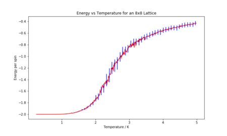
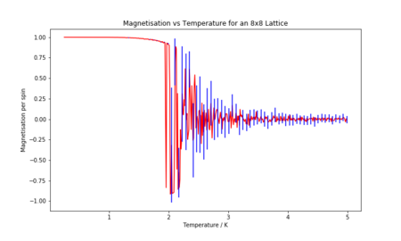
Simulations of 100,000 cycles were run every 0.01K from 0.25 to 5 K on an 8x8 Lattice. The plots of energy per spin vs temperature, and magnetisation per spin vs temperature, both with errorbars, are shown below.
 |
 |
The effect of system size
TASK: Repeat the final task of the previous section for the following lattice sizes: 2x2, 4x4, 8x8, 16x16, 32x32. Make sure that you name each datafile that your produce after the corresponding lattice size! Write a Python script to make a plot showing the energy per spin versus temperature for each of your lattice sizes. Hint: the NumPy loadtxt function is the reverse of the savetxt function, and can be used to read your previously saved files into the script. Repeat this for the magnetisation. As before, use the plot controls to save your a PNG image of your plot and attach this to the report. How big a lattice do you think is big enough to capture the long range fluctuations?
Plots were created in Jupyter Notebook, using the code below.

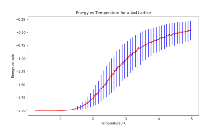
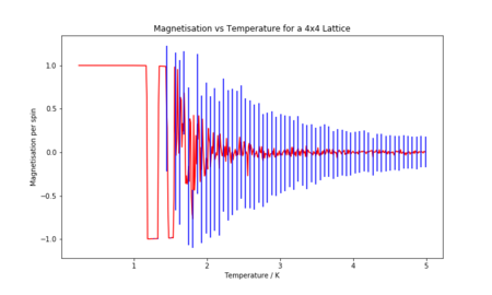
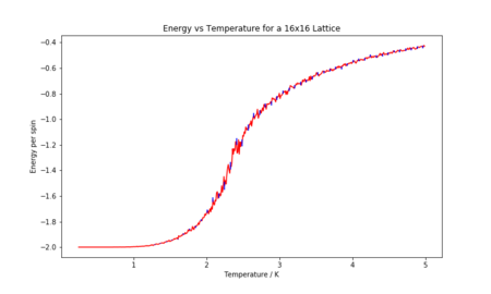
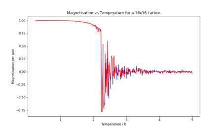
As lattice size gets larger, the error in the data gets smaller. I would say a 16x16 lattice is large enough to capture long range fluctuations. At the curie temperature, the energy should change almost instantaneously from -2 to the higher energy. The 16x16 lattice is when the energy curve begins to match this enough to be a reasonable approximation.
Determining the heat capacity
TASK: By definition,
C =
From this, show that
C =
(Where is the variance in E.)
Therefore
Leaving aside for now, we can analyse
As given before,
Where Z is the partition function,
It can be seen that
Taking each term in turn, starting with the first term;
Now taking the second term;
by the product rule. Therefore;
Therefore;
As seen before,
Combining and , gives
As , Variance can be substituted into this equation to give the desired result;
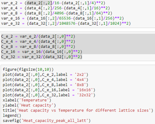
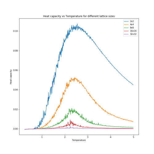
TASK: Write a Python script to make a plot showing the heat capacity versus temperature for each of your lattice sizes from the previous section. You may need to do some research to recall the connection between the variance of a variable, , the mean of its square , and its squared mean . You may find that the data around the peak is very noisy — this is normal, and is a result of being in the critical region. As before, use the plot controls to save your a PNG image of your plot and attach this to the report.
Locating the Curie temperature
For an infinite lattice size, the heat capacity diverges at the Curie temperature. However, with a finite lattice size the Curie temperature can be seen as a strong peak in heat capacity. The Curie temperature also changes with lattice size (finite size effect).
TASK: A C++ program has been used to run some much longer simulations than would be possible on the college computers in Python. You can view its source code here if you are interested. Each file contains six columns: T, E, E^2, M, M^2, C (the final five quantities are per spin), and you can read them with the NumPy loadtxt function as before. For each lattice size, plot the C++ data against your data. For one lattice size, save a PNG of this comparison and add it to your report — add a legend to the graph to label which is which. To do this, you will need to pass the label="..." keyword to the plot function, then call the legend() function of the axis object (documentation here).
 |
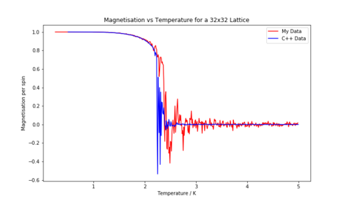 |
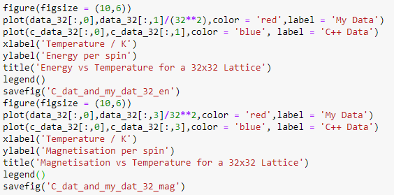
It can be seen that the data from C++ closely matches the data from my simulation, however the C++ data for energy is a smoother curve- due to more montecarlo steps resulting in less error in average energy. The C++ data for magnetisation shows earlier divergence from permanent magnetisation. The script used to plot this is shown below.
Polynomial Fitting
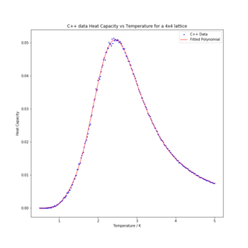
TASK: write a script to read the data from a particular file, and plot C vs T, as well as a fitted polynomial. Try changing the degree of the polynomial to improve the fit — in general, it might be difficult to get a good fit! Attach a PNG of an example fit to your report.
The code used for fitting a polynomial (order 30) to the heat capacity data for a 16x16 lattice is shown below.

It is difficult to get a good fit using this method. Smaller lattice sizes are relatively easy to fit, but lattice sizes over 4x4 become almost impossible to fit well.
Fitting in a particular temperature range
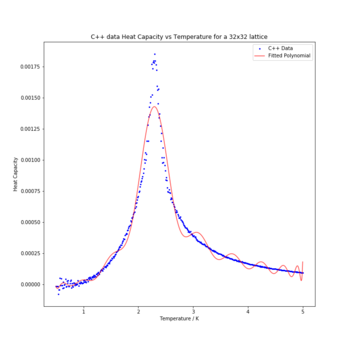
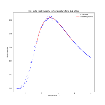
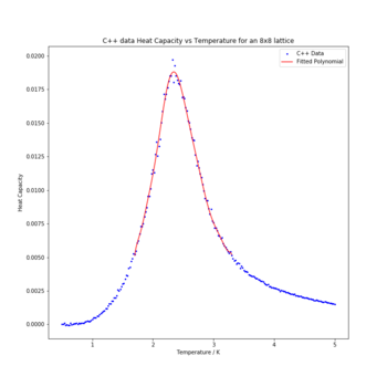
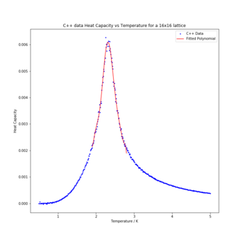
TASK: Modify your script from the previous section. You should still plot the whole temperature range, but fit the polynomial only to the peak of the heat capacity! You should find it easier to get a good fit when restricted to this region.
The selection of data within the array that corresponded to each peak was selected by trial and error. The code for fitting only the peak and plotting the result for the 32x32 Lattice is shown below.

Restricting to the peak region made it far easier to get a good fit, as shown below.
 |
 |
 |
 |
 |
 |
Finding the peak in C
TASK: find the temperature at which the maximum in C occurs for each datafile that you were given. Make a text file containing two colums: the lattice side length (2,4,8, etc.), and the temperature at which C is a maximum. This is your estimate of TC for that side length. Make a plot that uses the scaling relation given above to determine . By doing a little research online, you should be able to find the theoretical exact Curie temperature for the infinite 2D Ising lattice. How does your value compare to this? Are you surprised by how good/bad the agreement is? Attach a PNG of this final graph to your report, and discuss briefly what you think the major sources of error are in your estimate.
The temperature at which the maximum in C occurred, along with the corresponding lattice size, was recorded in the datafile Curie Temperature for different lattice sizes linked here.
The scaling relation for Curie temperature is , where is the Curie temperature of an lattice, is the Curie temperature of an infinite lattice, and A is a constant.
A curvefit was used to fit the data above to this scaling relation. The code for carrying out the fit and plotting the fit against the data is shown below.
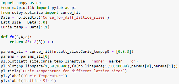

From the curvefit, the value for can be extracted and is found to equal 2.279 K (4 s.f.). The theoretical exact curie temperature for the infinite 2D Ising Lattice has been calculated to be equal to 2.269 K (4 s.f.)1. My calculated value is surprisingly close to the theoretical exact value, considering the scaling relation plot has only been generated using 6 datapoints. From observing this plot, it is clear that the datapoints do not lie exactly along the curvefit plotted, and inaccuracy in the curvefit is likely a large source of error. There are minor errors throughout in peak fitting and variations in energy from montecarlo, which may result in datapoints not lying exactly on the correct relation curve, however with more datapoints (i.e. more lattice sizes) the relation curve could be more accurately generated and thus the value for calculated more accurately.
References
[1] Exact 2D Ising Lattice Curie Temperature

