Rep:CMB1517-CMP-IsingModel

Introduction to the Ising Model

The Model

Figure1: 1D, 2D and 3D representations of the lattices in the Ising model.

The Ising model is a statistical model used to investigate and display the paramagnetic-ferromagnetic phase transition behaviour in ferromagnets. In other words, the spontaneous process of magnetisation in the absence of an external field as the temperature decreases past a certain temperature known as the Curie Temperature. We can think of all the atoms in a solid as having their own magnetic moment which contribute to the overall magnetic moment of the material. If these magnetic moments on the atoms in the solid are coupled to one another then as the temperature decreases there will be spontaneous ordering of the magnetic moments to the most stable ground state configuration and if this ordering results in all the magnetic moments being aligned and parallel to one another the material is said to be ferromagnetic.

In the Ising model we consider a chain of sites in 1D, an (N x N) lattice of sites in 2D, an (N x N x N) cube of sites in 3D and so on where each site $i$ is occupied by a so-called spin, $s_i$, this can be illustrated in Figure1. The magnetic dipole interactions restrict the spins to line parallel or anti-parallel along a given direction in uniaxial magnetic materials and so the spins can either be spin up $s_i=+1$ or spin down $s_i=-1$, by convention spin up is assigned to be positive.

There is a balance between an energetic driving force (which seeks to minimise the energy of the entire system by finding a configuration in which all spins are parallel) and an entropic driving force which is temperature dependent (which seeks to maximise the entropy of the system by finding a configuration in which all the spins alternate going from one site to another). This is encapsulated in the equation below,

$F=⟨E⟩-TS$

In the Ising model every spin can interact with its nearest neighbours as either a favoured interaction when both spins are parallel $\uparrow \uparrow$ or an unfavourable interaction when the spins are antiparallel $\uparrow \downarrow$. By convention we define the favoured interaction energy as negative $-J_{ij}$ and the unfavored interaction as positive $+J_{ij}$, hence why we have a negative sign in-front of the formula for the total energy of the lattice which is given by Equation 1. Note also that the spins on the lattice edges also interact with the spins on the other-side.

$E_{\alpha }=-\frac{1}{2}J\sum _i^N\sum _{j\in \text{ neignbours }(i)}{s}_i{s}_j$ - [1]

Where $J$ determines the strength of the interactions between the two spins and the factor of a half takes into account that we do not count each interaction twice as we iterate over all of the lattice sites.

TASK: Show that the lowest possible energy for the Ising model is $E=-DNJ$, where $D$ is the number of dimensions and $N$ is the total number of spins. What is the multiplicity of this state? Calculate its entropy.

To understand where this equation comes from lets simplify our problem to a 1D case where we will have a N sized chain of lattice sites that each contain a spin. We know that the minimum energy will be when all the spins are either spin up $s_i=+1$ or spin down $s_i=-1$ and this will be favoured at small temperatures as the thermal energy can't overcome the energetic barrier required to flip a state.

1D

We know the total energy is a model is given by Equation 1. In one dimension each spin has two neighbours and therefore two interactions per spin so the energy contribution from any one spin is given by,

$\begin{array}{r}{E}_{spin}=-\frac{1}{2}J[(+1)(+1)+(+1)(+1)]=-J\end{array}$

Therefore the total energy of the system is given by summing the energy over all sites,

$\begin{array}{r}{E}_{total}=E_{spin1}+E_{spin2}+E_{spin3}+...+E_{spinN}=-NJ\end{array}$

2D

If we move to two dimensions each spin now has 4 immediate neighbours and thus 4 interactions per spin in the lattice and so by the same logic as for the 1D case,

$\begin{array}{rl}{E}_{spin}& =-\frac{1}{2}J[(+1)(+1)+(+1)(+1)+(+1)(+1)+(+1)(+1)]=-2J\\ E_{total}& =E_{spin1}+E_{spin2}+E_{spin3}+...+E_{spinN}=-2NJ\end{array}$

3D

In three dimensions each spin now has 6 immediate neighbours and thus 6 interactions per spin the lattice and so by the same logic,

$\begin{array}{rl}{E}_{spin}& =-\frac{1}{2}J[(+1)(+1)+(+1)(+1)+(+1)(+1)+(+1)(+1)+(+1)(+1)+(+1)(+1)]=-3J\\ E_{total}& =E_{spin1}+E_{spin2}+E_{spin3}+...+E_{spinN}=-3NJ\end{array}$

It is evident that we have a well defined relationship between the dimensionality of the lattice and the number of interactions per spin to be $No.Interactions=2D$ arising thus we end up with $E=-DNJ$

Alternatively as all spins are either spin up $s_i=+1$ or spin down $s_i=-1$ we always know that $s_i{s}_j=+1$ for both cases and for all interactions within the lattice and thus we can say,

$\begin{array}{r}{E}_{\alpha }=-\frac{1}{2}J\sum _i^N\sum _{j\in \text{ neignbours }(i)}{s}_i{s}_j=-\frac{1}{2}J\sum _i^N\sum _{j\in \text{ neignbours }(i)}1\\ \end{array}$

we know that for a general dimension D the number of interactions per spin site will be 2D and hence our sum in j will be bounded by 2D interactions.

$\begin{array}{rl}{E}_{\alpha }& =-\frac{1}{2}J\sum _i^N\sum _{j\in \text{ neignbours }(i)}^{2D}1\\ & =-\frac{1}{2}J\sum _i^{N}2D=-\frac{2DNJ}{2}=-NDJ\end{array}$

Multiplicity

Multiplicity is defined as the total number of ways a state can be configured. For a system of size $N$ with states $n_1,n_2,...n_n$ where each state is indistinguishable from itself but distinguishable from the other states the number of permutations (multiplicity) $\mathrm{\Omega }$ is given by Equation 2

$\begin{array}{r}\mathrm{\Omega }=\frac{N!}{n_1!n_2!...n_n!}\end{array}$ - [2]

For our Ising model we have $N$ spins with possible states $$\begin{gathered} n_{\uparrow } \\ and \\ {n}_{\downarrow } \end{gathered}$$ and thus the multiplicity can be given by,

$\begin{array}{r}\mathrm{\Omega }=\frac{N!}{n_{\uparrow }!n_{\downarrow }!}\end{array}$

For the lowest energy state of the lattice all the spins are parallel to one another and so this can only happen in one particular configuration however because the spins can either be spin up $\uparrow$ or spin down $\downarrow$ ,which are of course degenerate configurations we have to include a degeneracy factor of 2.

$\begin{array}{r}\mathrm{\Omega }=degeneracy\times \frac{N!}{n_{\uparrow }!n_{\downarrow }!}=2\times \frac{N!}{N!0!}=2\end{array}$

Therefore the lowest energy configuration has a multiplicity of 2.

Entropy

In order to calculate the entropy of the system we need to introduce the Boltzman Law which defines entropy as a function of multiplicity given by Equation 3

$\begin{array}{r}S=k_b\ln \mathrm{\Omega }\end{array}$ - [3]

where $k_b$ is the Boltzmann constant $1.38064852\times 10^{23}J{K}^{-}1$.

Therefore plugging in our value of $\mathrm{\Omega }=2$,

$\begin{array}{r}S=k_b\ln 2=9.57\times 10^{-24}J{K}^{-1}\end{array}$

Phase Transitions

As said previously the Ising model allows us to see the paramagnetic-ferromagnetic phase transition at the Curie Temperature. The distribution of the spins is dependent on the temperature of the system as at low temperatures the thermal energy is not great enough to overcome the energetic stability gained by having all the spins parallel to one another, the energetic driving force dominates and we observe a organised magnetised phase. As we go to higher temperatures the thermal energy can overcome this barrier and start changing the spin states, thus trying to achieve maximum entropy of the system which would occur when the spins alternate from one site to another, which means we would observe a disordered magnetised phase.

TASK: Imagine that the system is in the lowest energy configuration. To move to a different state, one of the spins must spontaneously change direction ("flip"). What is the change in energy if this happens ($D=3,N=1000$)? How much entropy does the system gain by doing so?

In three dimensions, any one spin state has 6 neighbours in the model and so if we change the spin state from $s_i=+1$ to $s_i=-1$ what would have been $-6J_{ij}$ contributing to the total energy of the system is now $+6J_{ij}$. Thus the total change in energy will be $\mathrm{\Delta }E=+12J_{ij}$

We can also show this more quantitively as we know that the minimum energy of the system in any dimension D is given by,

$\begin{array}{r}{E}_{before}=-NDJ\end{array}$

If we can use Equation 1 to calculate what the energy would be if we flipped one spin where we consider the whole lattice before flipping giving rise to the $2ND$ term. Taking out that spin giving rise to the $4D$ term as we are loosing essentially$4D$ interactions if we are counting from the perspective of the spin that flipped and then double that as we count for each immediate neighbour. We then put the spin back being flipped giving rise to the second $4D$ gaining $4D$ unfavored interactions.

$\begin{array}{rl}{E}_{after}& =-\frac{1}{2}J[2ND-4D-4D]=4DJ-DNJ\\ \end{array}$

Thus we can work out the change in energy,

$\begin{array}{rl}\mathrm{\Delta }E& =E_{after}-E_{before}=4DJ-DNJ+DNJ=4DJ\end{array}$

When $D=3$

$\begin{array}{r}\mathrm{\Delta }E=+12J\end{array}$

Using the formula we derived earlier we can calculate what the energy of the system would have been for the ground state,

$\begin{array}{r}{E}_{\alpha }=-NDJ=-1000\times 3\times J=-3000J\end{array}$

And if we were to flip one spin state in the system this would create a change in energy of $\mathrm{\Delta }E=+12J_{ij}$ and hence,

$\begin{array}{r}{E}_{\alpha new}=-3000J+12J=-2988J\end{array}$

To work out the change in entropy of the system by flipping one spin recall that the entropy of the lowest configuration is given by,

$\begin{array}{r}S=k_b\ln 2\end{array}$

We can calculate the multiplicity for the system after we flip one spin to be,

$\begin{array}{r}\mathrm{\Omega }=degeneracy\times \frac{N!}{n_{\uparrow }!n_{\downarrow }!}=2\times \frac{1000!}{999!1!}=2000\end{array}$

and thus the entropy after is,

$\begin{array}{r}S=k_b\ln 2000\end{array}$

therefore the change in entropy is,

$\begin{array}{rl}\mathrm{\Delta }S& =S_{after}-S_{before}\\ & =k_b\ln 2000-k_b\ln 2\\ & =k_b\ln \frac{2000}{2}\\ & =k_b\ln 1000=9.54\times 10^{-23}J{K}^{-1}\end{array}$

TASK: Calculate the magnetisation of the 1D and 2D lattices in figure 1. What magnetisations would you expect to observe for an Ising lattice with $D=3,N=1000$ at absolute zero?

We can characterise the total magnetisation of the system by taking a linear sum of the individual spins across the entire system, this is given by Equation 4

$\begin{array}{r}{M}_{\alpha }=\sum _i{s}_i\end{array}$ - [4]

Referring back to Figure 1 for the 1D and 2D cases we can simply sum up the spins to figure out the magnetisation of the system using Equation 4

$\begin{array}{rl}{M}_{1D}& =\sum _i{s}_i=[(+1)+(+1)+(+1)+(-1)+(-1)]=+1\\ M_{2D}& =\sum _i{s}_i=[13\times (+1)+12\times (-1)]=+1\end{array}$

For a system with 1000 spins at 0K we would expect the energy of the system to be in the ground state and thus all the spins would be aligned with one another and so if we summed over all the spins then we could get two possible answers depending on weather the spins are aligned spin up $\uparrow$ or spin down $\downarrow$

$$\begin{gathered} \begin{array}{rl}M& =\sum _i{s}_i=[1000\times (+1)]=+1000\\ M& =\sum _i{s}_i=[1000\times (-1)]=-1000\\ hence \\ M& =\sum _i{s}_i=\pm 1000\end{array} \end{gathered}$$

Calculating the Energy and Magnetisation

Modifying the files

TASK: complete the functions energy() and magnetisation(), which should return the energy of the lattice and the total magnetisation, respectively. In the energy() function you may assume that $J=1.0$ at all times (in fact, we are working in reduced units in which $J=k_B$, but there will be more information about this in later sections). Do not worry about the efficiency of the code at the moment — we will address the speed in a later part of the experiment.

Writing the energy() function: Initial thoughts were to loop through every lattice site calculate all four interactions and add them each to the total energy and then divide by 2 at the end, however this quickly led to complications when you got to the end of the array as an additional increase in the loop did not wrap around to the start and required a lot of hardcoding for each explicit case. Instead I realised that instead of dividing by 2 at the end we could instead just calculate the same two interactions for every lattice point. To fix the wrap around problem for the arrays we can introduce a mod function which essentially takes care of this for us.

def energy(self):
        "Return the total energy of the current lattice configuration."

        #initialise the energy variable to 0
        energy = 0.0

        #loop through every row
        for i in range(self.n_rows):
            #loop through every coloumn in the row
            for j in range(self.n_cols):

                #for every spin add the energy of the interactions on the right and below
                energy = energy - (self.lattice[i][j] * self.lattice[(i+1)%self.n_rows][j]
                                   + self.lattice[i][j] * self.lattice[i][(j+1)%self.n_cols])
        return energy

Writing the magnetisation() function: The magnetisation function was much simpler to implement as we just had to loop through all the spins in the lattice and add their values to the magnetisation variable.

def magnetisation(self):
        "Return the total magnetisation of the current lattice configuration."

        #initialise the magnetisation variable to 0
        magnetisation = 0

        #loop through every row
        for i in range(self.n_rows):
            #loop through every row
            for j in range(self.n_cols):
                
                #for every spin add the spin value to the magnetisation variable
                magnetisation = magnetisation + self.lattice[i][j]
                
        return magnetisation

Testing the files

TASK: Run the ILcheck.py script from the IPython Qt console using the command

%run ILcheck.py

The displayed window has a series of control buttons in the bottom left, one of which will allow you to export the figure as a PNG image. Save an image of the ILcheck.py output, and include it in your report.

Figure2: Figure illustrating that the energy() and magnetisation() functions work.

The script generates plots for each of a perfectly ordered system, a perfectly disordered system and also a random system and calculates expected values and checks against values produced by my own implemented energy() and magnetisation() functions. It is evident from the checking script that the implemented functions are correct.

Introduction to Monte Carlo simulation

Average Energy and Magnetisation

In the Ising model we are particular interested in finding the values for the energy of the system and also the magnetisation of the system so we need to introduce the statistical equations that model these quantities, Equation 4 and Equation 5, give the average total magnetisation and average total energy respectively where Z Is the partition function which is a weighted average over all the micro states in a system.

$⟨M{⟩}_T=\frac{1}{Z}\sum _{\alpha }M(\alpha )\exp \{-\frac{E(\alpha )}{k_{B}T}\}$ - [4]

$⟨E{⟩}_T=\frac{1}{Z}\sum _{\alpha }E(\alpha )\exp \{-\frac{E(\alpha )}{k_{B}T}\}$ - [5]

$Z=\sum _{\alpha }\exp \{-\frac{E(\alpha )}{k_{B}T}\}$ - [6]

TASK: How many configurations are available to a system with 100 spins? To evaluate these expressions, we have to calculate the energy and magnetisation for each of these configurations, then perform the sum. Let's be very, very, generous, and say that we can analyse $1\times 10^9$ configurations per second with our computer. How long will it take to evaluate a single value of ${⟨M⟩}_T$?

Every lattice site can either accommodate a spin to be spin up (+1) or spin down (-1) and so for every site we have 2 choices therefore there are are 2 to the power of 100 configurations,

$\mathrm{\Omega }=2^{100}$

If we make the assumption that a computer can compute $10^9$ configurations every second then to calculate $2^{100}$ configurations it would take,

$$\begin{gathered} t=\frac{2^{100}}{10^9}=1.27\times 10^{21}s=402714358194 \\ centuries \end{gathered}$$

This is way too long and practically impossible to calculate.

For a large proportion of the configurations where the energy will be really close to zero the Boltzmann factor is going to be a very small number and if we think about this contribution of that product to the entire summation of all the other configurations then it is essentially going to make a small difference to the value and we can ignore it. This is known as the concept of importance sampling.

Importance Sampling

Figure3: Figure illustrating the Monte Carlo Algorithm for the Ising Model

We want to make sure we are using samples from the interesting and important parts for our statistical calculations. This can be achieved by sampling from a distribution in which over weights in region of interest. In order to do this we introduce the Monte Carlo algorithm. This allows us to randomly generate states from then Boltzman distribution which will now solve our problem.

Looking at Figure 3 we can see how the algorithm works:

1. Start from a given system comprised of a lattice of spins ${\alpha }_{\alpha }$ with total energy $E_{\alpha }$
2. Randomly flip a spin in the system to create a new one ${\alpha }_{\beta }$
3. Recalculate the energy for this new system $E_{\beta }$
4. Calculate the difference in energy between the two spin systems $\mathrm{\Delta }E=E_{\beta }-E_{\alpha }$
   1. If $\mathrm{\Delta }E<0$ meaning that the new system has decreased the energy, then we accept the new configuration.
      • We set ${\alpha }_{\alpha }={\alpha }_{\beta }$ and $E_{\alpha }=E_{\beta }$, and then go to step 5
   2. If $\mathrm{\Delta }E>0$ meaning that the new system has increased the energy, then we need to consider the probability of actually seeing the two states ${\alpha }_{\alpha }$ and ${\alpha }_{\beta }$. It can be shown that the probability for the transition between the two to occur is $\exp (-\frac{\mathrm{\Delta }E}{k_{B}T})$ and to make sure that we only accept this kind of spin flip with the correct probability, we use the following procedure:
      1. Choose a random number $R$ in the interval $[0,1)$
      2. If $R<=\exp (-\frac{\mathrm{\Delta }E}{k_{B}T})$, we accept the new configuration,
         • We set ${\alpha }_{\alpha }={\alpha }_{\beta }$ and $E_{\alpha }=E_{\beta }$, and then go to step 5
      3. If $R>=\exp (-\frac{\mathrm{\Delta }E}{k_{B}T})$, we reject the new configuration,
         • ${\alpha }_{\alpha }$ and $E_{\alpha }$, are left unchanged and we go to step 5
5. Update the running averages of the energy and magnetisation
6. Return to step 2

We can see that in step 4 we only accept new configurations that increase the energy of the system if they have the right probability and so we are excluding any transitions that would be highly unlikely and thus not give any real value to the average of the energy and magnetisation that we are trying to work out.

Modifying IsingLattice.py

TASK: Implement a single cycle of the above algorithm in the montecarlocycle(T) function. This function should return the energy of your lattice and the magnetisation at the end of the cycle. You may assume that the energy returned by your energy() function is in units of $k_B$! Complete the statistics() function. This should return the following quantities whenever it is called: $<E>,<E^2>,<M>,<M^2>$, and the number of Monte Carlo steps that have elapsed.

Writing the montecarlostep() function: Instead of having an "if" statement for every check in the algorithm it is only necessary to make one check to determine if we reject the new configuration thus increasing the efficiency of the algorithm. The values are then adding to the running sums at the end of every "Monte Carlo" step.

def montecarlostep(self, T):
        #calculate energy before
        energy_before = self.energy()
        
        #generate coordinates of the random spin
        random_i = np.random.choice(range(0, self.n_rows))
        random_j = np.random.choice(range(0, self.n_cols))

        #flip the spin value of the random spin
        self.lattice[random_i][random_j] *= -1

        #calculate the energy after and change in energy
        energy_after = self.energy()
        change_energy = energy_after - energy_before

        #random number in the range [0,1) generated
        random_number = np.random.random()

        #only way for the configuration to be rejected is if this condition is true
        if change_energy > 0 and random_number > np.e ** (-(change_energy / T)):

            #reject the configuration
            self.lattice[random_i][random_j] *= -1

        #update the running averages of the energy and magnetisation
        self.E += self.energy()
        self.E2 += (self.energy()) ** 2
        self.M += self.magnetisation()
        self.M2 += (self.magnetisation()) ** 2

        return self.energy(), self.magnetisation()

Writing the statistics() function:

def statistics(self):
        "returns the values for the averages of E, E2, M and M2"

        Ave_E = self.E / self.n_cycles
        Ave_E2 = self.E2 / self.n_cycles
        Ave_M = self.M / self.n_cycles
        Ave_M2 = self.M2 / self.n_cycles
        Cycles = self.n_cycles

        return Ave_E, Ave_E2, Ave_M, Ave_M2, Cycles

TASK: If $T<T_C$, do you expect a spontaneous magnetisation (i.e. do you expect $⟨M⟩\ne 0$)? When the state of the simulation appears to stop changing (when you have reached an equilibrium state), use the controls to export the output to PNG and attach this to your report. You should also include the output from your statistics() function.

• 

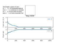
  Figure4: State of minimum energy

• 

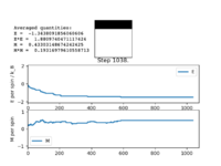
  Figure5: Local minimum found

• 

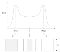
  Figure5.5: Local minimum representation

When $T<T_C$ you would be sure to expect spontaneous magnetisation as the thermal energy will be too small to overcome the energetic driving force trying to achieve a minimum energy state, this will result in the majority of the spins being aligned to one another and therefore $⟨M⟩\ne 0$ leading to spontaneous magnetisation as there will be a net magnetic dipole moment in one direction.

Figure 4 and Figure 5 are some images of the animations after around 1000 steps for an 8x8 lattice at a temperature of T=0.5 where the white represents a spin value of +1 and black a spin value of -1. In Figure 4 we can see that just after 200 steps the model converged to its ground state energy and thus every trial spin flip from there on was rejected. We can also see the average values of the simulation that have been skewed due to the initial period at the start where there was a decay in energy. Imagining we are on a potential energy surface then Figure 5 shows a simulation that has found a local minima where it has formed a group of spin up sites and a group of spin down sites.

Accelerating the code

TASK: Use the script ILtimetrial.py to record how long your current version of IsingLattice.py takes to perform 2000 Monte Carlo steps. This will vary, depending on what else the computer happens to be doing, so perform repeats and report the error in your average!

1	2	3	4	5	Mean	Standard Mean Error
31.33	32.13	31.07	31.57	33.30	31.88	0.396

TASK: Look at the documentation for the NumPy sum function. You should be able to modify your magnetisation() function so that it uses this to evaluate M. The energy is a little trickier. Familiarise yourself with the NumPy roll and multiply functions, and use these to replace your energy double loop (you will need to call roll and multiply twice!).

Instead of summing over all the spins in the lattice we can simply use np.sum() which will do it for us in the idea that the numpy module has many operations implemented in C that avoid the general cost of loops in python. Instead of using a double for loop to go through all the values in the lattice and calculate the energies for all spins we can now use the np.roll() function to multiply the original lattice by rolling it in the x direction and adding this to the product of the original lattice and rolling it in y direction. This is essentially the same as looping through all values but without the cost of using a computational expensive double for loop. A few additional changes were also made to the code. First of all instead of adding the values of each cycle to a running some and then having to divide these values at the end I thought it would be much more useful to add these values to a list which will store all the values and we can then simply use the optimised NumPy functions to calculate the mean of these lists at the end in the statistics function. Secondly we were calling the self.energy() function a lot within the Monte Carlo step function which then in turn will run the function but instead of this it seems much better to define an attribute native to the class of the current energy which can store the value and thus we only need to call a set value rather than a function every time we need to use it.

import numpy as np

class IsingLattice:

    E = []
    E2 = []
    M = []
    M2 = []

    n_cycles = 1

    def __init__(self, n_rows, n_cols):
        self.n_rows = n_rows
        self.n_cols = n_cols
        self.lattice = np.random.choice([-1,1], size=(n_rows, n_cols))
        self.current_energy = self.energy()

    def energy(self):
        "Return the total energy of the current lattice configuration."

        energy = -np.sum(self.lattice * np.roll(self.lattice, 1, 1) + self.lattice * np.roll(self.lattice, 1, 0))
    
        return energy

    def magnetisation(self):
        "Return the total magnetisation of the current lattice configuration."

        magnetisation = np.sum(self.lattice)
                
        return magnetisation

    def montecarlostep(self, T):
        
        #generate coordinates of the random spin
        random_i = np.random.choice(range(0, self.n_rows))
        random_j = np.random.choice(range(0, self.n_cols))

        #flip the spin value of the random spin
        self.lattice[random_i][random_j] *= -1

        #calculate the energy after and change in energy
        energy_after = self.energy()
        change_energy = energy_after - self.current_energy

        #random number in the range [0,1) generated
        random_number = np.random.random()

        #only way for the configuration to be rejected is if this condition is true
        if change_energy > 0 and random_number >= np.e ** (-(change_energy / T)):

            #reject the configuration
            self.lattice[random_i][random_j] *= -1
        else:
            #accept the configuration
            self.current_energy = self.energy()

        #add the values to the arrays
        self.E.append(self.current_energy)
        self.E2.append(self.current_energy**2)
        self.M.append(self.magnetisation())
        self.M2.append(self.magnetisation()**2)
        self.n_cycles += 1

        return self.current_energy, self.magnetisation()

    def statistics(self):
        "returns the values for the averages of E, E2, M and M2"

        return np.mean(self.E), np.mean(self.E2), np.mean(self.M), np.mean(self.M2)

TASK: Use the script ILtimetrial.py to record how long your new version of IsingLattice.py takes to perform 2000 Monte Carlo steps. This will vary, depending on what else the computer happens to be doing, so perform repeats and report the error in your average!

1	2	3	4	5	Mean	Standard Mean Error
0.18	0.21	0.20	0.20	0.20	0.198	0.0043

After optimising the script we can see an improvement of 160 times faster!

The effect on temperature

Correcting the average code

As we saw before in Figure 4 and Figure 5 the average values of the energy and magnetisation (per spin) are not -2 or either +/- 1 as we would of expected due to the initial decay in energy and magnetisation as the system gets to a stable state and then starts to equilibrate and the values taken into account in the average from the start are skewing the statistics.

TASK: The script ILfinalframe.py runs for a given number of cycles at a given temperature, then plots a depiction of the final lattice state as well as graphs of the energy and magnetisation as a function of cycle number. This is much quicker than animating every frame! Experiment with different temperature and lattice sizes. How many cycles are typically needed for the system to go from its random starting position to the equilibrium state? Modify your statistics() and montecarlostep() functions so that the first N cycles of the simulation are ignored when calculating the averages. You should state in your report what period you chose to ignore, and include graphs from ILfinalframe.py to illustrate your motivation in choosing this figure.

Varying lattice sizes at a constant temperature

• 

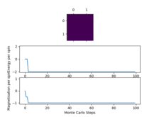
  Figure6: 2x2, T=1

• 

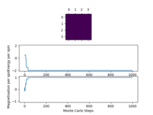
  Figure7: 4x4, T=1

• 

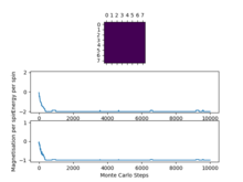
  Figure8: 8x8, T=1

• 

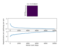
  Figure9: 16x16, T=1

• 

  Figure10: 32x32, T=1

We can see that as we increase the system size the "cut off" point for when the system reaches a state of equilibrium increases as it takes more and more Monte Carlo steps in order for the system to get to its lowest energy configuration as there are more spins to flip in order to reach this point.

Varying temperature at a constant lattice size

• 

  Figure11: 8x8, T=1

• 

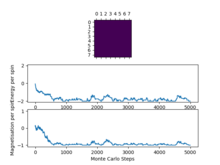
  Figure12: 8x8, T=2

• 

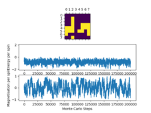
  Figure13: 8x8, T=3

• 

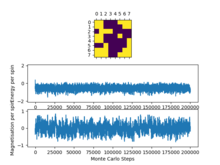
  Figure14: 8x8, T=4

• 

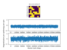
  Figure15: 8x8, T=5

We can see that keeping the system size constant and increasing the temperature for temperatures that are below the Curie temperature take longer in this case however I think weather or not an increase in temperature below the curie temperature will increase the time taken to reach equilibrium depends on how far away from the curie temperature you are, as in some cases it may take longer as there is more of an entropic contribution resisting the energetic driving force however it could also increase the time it takes as the system has more energy and can flip spins more quickly in order to reach that ground state energy. At temperatures above the curie temperature the entropic driving force dominates and the system does not reach a stable ground state but still reaches a thermal equilibrium.

It is clear that these both have an effect on the "cut off" point and so a different point will need to be selected for different conditions. An alternative would be to try to implement an auto detecting algorithm that would only start counting if the gradient of the average of a set of points is within a certain threshold close to 0.

Below are the values I decided to use for the cut off points.

2x2	4x4	8x8	16x16	32x32
8	250	2000	8000	120000

Because I appended the average energy values into a list I could simply define a new statistics function that returned the values in a list after a certain cut off point using list slicing instead of having to put an if statement into the Monte Carlo step function that would of been computationally more expensive. Downside to this method is that we are storing values that are not needed and so it is memory expensive.

Modified statistics() function:

 def statistics2(self,cut_off):
        "returns the values for the averages of E, E2, M, M2, stdE, stdM only taking into account the cutoff"

        return np.mean(self.E[cut_off:]), np.mean(self.E2[cut_off:]),
                   np.mean(self.M[cut_off:]), np.mean(self.M2[cut_off:]),
                   np.std(self.E[cut_off:]), np.std(self.M[cut_off:])

Running over a range of temperatures

TASK: Use ILtemperaturerange.py to plot the average energy and magnetisation for each temperature, with error bars, for an $8\times 8$ lattice. Use your intuition and results from the script ILfinalframe.py to estimate how many cycles each simulation should be. The temperature range 0.25 to 5.0 is sufficient. Use as many temperature points as you feel necessary to illustrate the trend, but do not use a temperature spacing larger than 0.5. The NumPy function savetxt() stores your array of output data on disk — you will need it later. Save the file as 8x8.dat so that you know which lattice size it came from.

Figure16: 8x8 Average energy and magnetisation as a function of temperature $\mathrm{\Delta }T=0.01$

Plotted in Figure16 in dark blue are the average energies and magnetisations as a function of temperature and then in light blue are the error bars for the values. Looking at the average energies we can see the ferromagnetic-paramagnetic phase transition occurring. At lower temperatures the energetic driving force is dominant and the systems reaches the lowest energy state where all the spins are parallel with one another thus giving rise to the average energy per spin value of roughly 2. Once the temperature starts to increase we can see that average energy per spin is slowly rising as this means that in the same number of steps the system is not able to reach the ground state configuration and the average values start to increase as entropy starts to play more of a role. We eventually get to the Curie Temperature, which is defined as the temperature above which magnetic materials lose their magnetic properties. This is the point where the phase transition takes place and now the temperature is great enough such that the thermal energy is sufficient to ignore the energetic barrier and entropy is dominant now, we start to observe some small oscillatory behaviour in this region as we have increased the temperature enough such that more spin flips are being accepted and so there are more possible states that the simulation can end with in the given number of steps hence in some cases the final state will be slightly more or less energetic than the region before but the general trend is that increasing the temperature increases the average energy.

Looking at the average magnetisations we can see that at lower temperatures below the Curie temperature the average magnetisation is at 1 with no negligible fluctuation as the thermal noise is weak. Once we start approaching the Curie temperature we are not reaching ground state configurations but are somewhat close(where the spins are mostly aligned with one another either in the up or down direction) which is why the magnitude of the oscillations start to decay with increasing temperature. As we hit the Curie temperature and beyond when entropy is dominating and the system reaches equilibrium states in which are trying to achieve maximum entropy. The spins are close to being in a 50:50 ratio of spin up and spin down and so the average starts to tend to zero and the fluctuations become increasing less interactive such that we can consider essential a system of non interacting spins.

The error bars are representative of how much the values deviate from the average values. We can see that in the average energy as a function of temperature that at low temperatures the error bars are very small as we are always going to converge to the lowest energy state and we will not deviate from this. Once we start increasing the temperature the error bars start to increase as we are accepting more spin flips and hence there are more and more possible energy values that the final state in the system can reach which in turn alters variance of the values and increases the error. In the average magnetisations as a function of temperature we see the inverse of this and infact the error bars start to decrease as once we get to a high enough temperature the entropic driving force has taken over and the average magnetisation is tending to zero and so the errors decrease.

Effect of the system size

Scaling the system

TASK: Repeat the final task of the previous section for the following lattice sizes: 2x2, 4x4, 8x8, 16x16, 32x32. Make sure that you name each datafile that your produce after the corresponding lattice size! Write a Python script to make a plot showing the energy per spin versus temperature for each of your lattice sizes. Hint: the NumPy loadtxt function is the reverse of the savetxt function, and can be used to read your previously saved files into the script. Repeat this for the magnetisation. As before, use the plot controls to save your a PNG image of your plot and attach this to the report. How big a lattice do you think is big enough to capture the long range fluctuations?

• 

  Figure17: 2x2

• 

  Figure18: 4x4

• 

  Figure19: 8x8

• 

  Figure20: 16x16

• 

  Figure21: 32x23

• 

  Figure21: Comparison

As before we can see the same trends of the average energy and magnetisation as a function of temperature. We can also see that the errors in both the average energy and average magnetisation decreases as the system size increases. The error bars are based of the standard deviation of the values and then divided by the number of spins in order to compare, the errors are representative of how much the average energy or magnetisation values fluctuate from the mean and so we are not surprised that once we increase the temperature the error bars also increase. We can also justify the fact that the errors decrease as we increase the system size as we have a larger sample and so we are dividing through by a larger number of total spins and so the errors decrease which essentially means that larger lattice sizes give a more accurate description of the model. Another important point to note is that comparing the average magnetisations for the different lattice sizes the temperature at which magnetisation is lost increases from the smaller lattice sizes until around an 8x8 lattice and as this is the definition of the Curie temperature then this means that the curie temperature increase up to this point. This is what we would expect as when we increase the system size there are more spins aligned with one another at lower temperatures and thus in-order to overcome a greater energetic barrier created at the lower temperatures a higher temperature is required. We can also see that in the overlapping comparisons in Figure 21 that the curves seem to converge after an 8x8 lattice size and that the range of fluctuations in magnetisation stop altering at this size too and only start fluctuating once the Curie temperature is reached whereas in the 2x2 and 4x4 lattice sizes the fluctuations start to occur way before the Curie temperature suggesting that an 8x8 lattice size is enough to capture long range fluctuations. In smaller lattice sizes as there are less spins then the effect of one spin flipping has an overall larger effect on the probability of flipping the whole system which is why we see the fluctuations at a lower temperature for the 2x2 and 4x4 lattice sizes.

Determining the heat capacity

Calculating the heat capacity

We now want to find a formula we can use to calculate the specific heat capacitie at a given temperature using the statistics that we have. We require the specific heat capacity in order to help us find the curie temperature.

TASK: By definition,

$C=\frac{\partial ⟨E⟩}{\partial T}$

From this, show that

$C=\frac{\mathrm{V}\mathrm{a}\mathrm{r}[E]}{k_B{T}^2}$

(Where $\mathrm{V}\mathrm{a}\mathrm{r}[E]$ is the variance in $E$.)

The derivation is as follows:

TASK: Write a Python script to make a plot showing the heat capacity versus temperature for each of your lattice sizes from the previous section. You may need to do some research to recall the connection between the variance of a variable, $\mathrm{V}\mathrm{a}\mathrm{r}[X]$, the mean of its square $⟨X^2⟩$, and its squared mean ${⟨X⟩}^2$. You may find that the data around the peak is very noisy — this is normal, and is a result of being in the critical region. As before, use the plot controls to save your a PNG image of your plot and attach this to the report.

Now that we have a formula for calculating the specific heat capacity we want to plot this against temperature in order to get a visual picture of roughly where the phase transition will take place.

The script used to plot the graphs was:

#initialises variables
temps = []
energies = []
magnetisations = []
energysq = []
magnetisationsq = []
heatCapacity = []

#loads data into variable
y = np.loadtxt('2x2.dat')

#seperated loaded data into variables
temps = y[:,0]
energies = y[:,1]
energysq = y[:,2]
    
def heat_cap(var,T):
    "returns the heat capacity from a givent variance and temperature"
    return var/(T**2)

#calculates the specific heat capacity for every temperature
for i in range(len(temps)):
    var = energysq[i] - (energies[i])**2
    heatCapacity += [heat_cap(var,temps[i]) / 4]
    
#plots specific heat capacity  against temperature     
pl.plot(temps,heatCapacity,lw=1,c='b')
pl.ylim(0,0.5)
pl.xlim(0,5)
pl.xlabel("Temperature / $K$")
pl.ylabel("Specific Heat Capacity / $J \ K^{-1}$")
pl.margins(x=0)
pl.margins(y=0)
pl.savefig('2x2_Cv.png',dpi=500,bbox_inches='tight')
pl.show()

The plots are shown below.

• 

  Figure 22: 2x2

• 

  Figure 23: 4x4

• 

  Figure 24: 8x8

• 

  Figure 25: 16x16

• 

  Figure 26: 32x32

We can see that as we increase the size of the system the peaks start to get sharper and rise higher. The peaks are representing the phase transition that takes place and thus we can estimate the curie temperature from the peaks. We know that Onsager proved that for an infinite system the heat capacity diverges up to infinity at the curie temperature and we see a first order phase transition however because our system sizes are so small and finite we observe a maximum peak in our system and thus the specific heat capacity is bounded by a maximum. The finite system introduces systematic errors known as the finite size effect. We can also describe the plot in terms of the rate of change of entropy with temperature as,

$C=T\frac{\partial S}{\partial T}$

At lower temperatures when the energetic driving force is dominant there is a low change in the entropy of the system with temperature but as we start to increase the temperature coming up to the Curie temperature when the entropic driving force is competing and taking over the energetic contribution then the rate of change of entropy with temperature is maximum. Once we have increased the temperature past the Curie temperature when the entropic contribution is dominant and maximum then there is no more increase in entropy and hence the rate of change goes back to zero.

Locating the curie temperature

TASK: A C++ program has been used to run some much longer simulations than would be possible on the college computers in Python. You can view its source code here if you are interested. Each file contains six columns: $T,E,E^2,M,M^2,C$ (the final five quantities are per spin), and you can read them with the NumPy loadtxt function as before. For each lattice size, plot the C++ data against your data. For one lattice size, save a PNG of this comparison and add it to your report — add a legend to the graph to label which is which. To do this, you will need to pass the label="..." keyword to the plot function, then call the legend() function of the axis object (documentation here).

The simulations run in C++ offer much more accurate data as longer run times were allowed.

Comparison of the specific heat capacity and average energies and magnetisations using the C++ data and python data

• 

  Figure 27: 2x2

• 

  Figure 28: 4x4

• 

  Figure 29: 8x8

• 

  Figure 30: 16x16

• 

  Figure 31: 32x32

• 

  Figure 32: 2x2

• 

  Figure 33: 4x4

• 

  Figure 34: 8x8

• 

  Figure 35: 16x16

• 

  Figure 36: 32x32

• 

  Figure 37: 2x2

• 

  Figure 38: 4x4

• 

  Figure 39: 8x8

• 

  Figure 40: 16x16

• 

  Figure 41: 32x32

We can immediately see that in general the data fits are good especially at low temperatures and then at higher temperatures due to their being a lot more fluctuation the fits are slightly worse.

Polynomial fitting

TASK: write a script to read the data from a particular file, and plot C vs T, as well as a fitted polynomial. Try changing the degree of the polynomial to improve the fit — in general, it might be difficult to get a good fit! Attach a PNG of an example fit to your report.

• 

  Figure43: Figure illustrating the polynomial fitting to a 4x4 specific heat capacity plot

• 

  Figure42: Figure illustrating the polynomial fitting to a 32x32 specific heat capacity plot

From these two figures we can see that for the smaller system sizes the fits are better but for the larger system sizes we can see that increasing the degree of the polynomial even up to an order of 20 is not sufficient enough to get a good fit.

Script used to plot

#load data in & sort
data = np.loadtxt('C++_data/32x32.dat')
T = data[:,0]
C = data[:,5]

#fit the data
fit1 = np.polyfit(T,C,2)
fit2 = np.polyfit(T,C,4)
fit3 = np.polyfit(T,C,8)
fit4 = np.polyfit(T,C,16)
fit5 = np.polyfit(T,C,20)

#determne max and min values of T & create a range of T points
T_min = np.min(T)
T_max = np.max(T)
# T_min = 1
# T_max = 4
T_range = np.linspace(T_min, T_max, 1000)

#create a range of the fitted points
fitted_C_values1 = np.polyval(fit1, T_range)
fitted_C_values2 = np.polyval(fit2, T_range)
fitted_C_values3 = np.polyval(fit3, T_range)
fitted_C_values4 = np.polyval(fit4, T_range)
fitted_C_values5 = np.polyval(fit5, T_range)

#plot
pl.plot(T,C,linestyle='',marker='x',markersize='1',c='r')
pl.plot(T_range,fitted_C_values1,label='Order 2',lw='1',c='lightskyblue')
pl.plot(T_range,fitted_C_values2,label='Order 4',lw='1',c='skyblue')
pl.plot(T_range,fitted_C_values3,label='Order 8',lw='1',c='deepskyblue')
pl.plot(T_range,fitted_C_values4,label='Order 16',lw='1',c='steelblue')
pl.plot(T_range,fitted_C_values5,label='Order 20',lw='1',c='b')
pl.xlim(0,5)
pl.xlabel("Temperature / $K$")
pl.ylabel("Specific Heat Capacity / $J \ K^{-1}$")
pl.margins(x=0)
pl.margins(y=0)
pl.legend(loc='best')
pl.savefig('32x32_Polyfit_C++.svg',bbox_inches='tight')

pl.show()

Fitting a particular temperature range

TASK: Modify your script from the previous section. You should still plot the whole temperature range, but fit the polynomial only to the peak of the heat capacity! You should find it easier to get a good fit when restricted to this region.

The polynomials in the previous section were not sufficient to capture a good fitting on the peaks of the specific heat capacity curves which is required in-order to find the maximum values of the specific heat capacity. The script was modified slightly in-order to only fit the polynomial about a selected temperature range that captured the required peaked region of the curves. The degree of the polynomials was of order 2 for all the fits.

• 

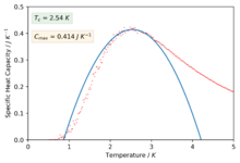
  Figure 43: 2x2

• 

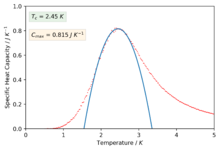
  Figure 44: 4x4

• 

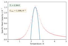
  Figure 45: 8x8

• 

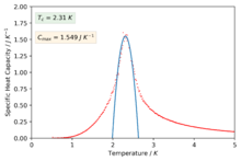
  Figure 46: 16x16

• 

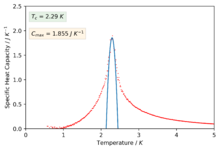
  Figure 47: 32x32

We can now see much better fitting to the interesting regions of the curve and we have also found values for the maximum of specific heat capacities and the temperatures at which they occur (our estimate for the Curie temperature).

Script used to plot:

#load data in & sort
data = np.loadtxt('C++_data/2x2.dat')
T = data[:,0]
C = data[:,5]

#determine max and min values of T & create a range of T points
T_min = 2.2
T_max = 2.9

#make a selection of only the values in the temp range
selection = np.logical_and(T > T_min, T < T_max)

#create range of selected data only
peak_T_values = T[selection]
peak_C_values = C[selection]

#fit the data 
fit = np.polyfit(peak_T_values, peak_C_values, 2)
# T_range = np.linspace(T_min, T_max, 1000)
T_range = np.linspace(np.min(T), np.max(T), 1000)

#create range of fitting values
fitted_C_values = np.polyval(fit, T_range)

#plot
pl.plot(T,C,linestyle='',marker='x',markersize='1',c='r')
pl.plot(T_range,fitted_C_values)
pl.xlim(0,5)
pl.ylim(0,0.5)
pl.xlabel("Temperature / $K$")
pl.ylabel("Specific Heat Capacity / $J \ K^{-1}$")
pl.margins(x=0)
pl.margins(y=0)
pl.text(0.15,0.45,r'$T_c$ = $2.54\ K$',bbox=dict(facecolor='g', alpha=0.10))
pl.text(0.15,0.38,r'$C_{max}$ = $0.414\ J \ K^{-1}$',bbox=dict(facecolor='orange', alpha=0.10))
# pl.text(3.5, 0.4, r'$T_{C, L} = \frac{A}{L} + T_{C,\infty}$')
# pl.legend(loc='best')
pl.savefig('cmb_2x2_Polyfit2_C++.png',dpi=500,bbox_inches='tight')

pl.show()

Finding the peak in C

TASK: find the temperature at which the maximum in C occurs for each datafile that you were given. Make a text file containing two colums: the lattice side length (2,4,8, etc.), and the temperature at which C is a maximum. This is your estimate of $T_C$ for that side length. Make a plot that uses the scaling relation given above to determine $T_{C,\mathrm{\infty }}$. By doing a little research online, you should be able to find the theoretical exact Curie temperature for the infinite 2D Ising lattice. How does your value compare to this? Are you surprised by how good/bad the agreement is? Attach a PNG of this final graph to your report, and discuss briefly what you think the major sources of error are in your estimate.

Figure 49: Tc plotted against 1/L with a linear fit

Using the Equation 7 we can use our estimated values of the Curie temperature found by fitting the polynomials on the peaks of the specific heat capacity curve for each system size to get a estimated value for the curie temperature for an infinite lattice size by simply plotting the Curie temperature against 1/L and performing a linear fit to extract the values for the gradient and intercepts. This analytic solution was found by Lars Onsager.

$T_{C,L}=\frac{A}{L}+T_{C,\mathrm{\infty }}$ -[7]

The value found from this plot was,

$T_{C,L}=2.28171922K\pm 0.1\mathrm{\%}$

and the value for A was, $A=0.53608447\pm 0.7\mathrm{\%}$

The result found by Onsager was,

$\frac{2}{\ln (1+\sqrt{2})}\approx 2.26918531$

So there is a percentage different of roughly 0.55%. A source of error to consider may be that the functions that we were fitting to is not a polynomial and gets less so as you increase the system size too. The real solution at an infinite lattice size diverges to infinity and it is clear that in tending to this limit a polynomial fit isn't going to be able to model a divergence however it is the best we can do. Perhaps another source of error comes from the fact that we showed that the smaller lattice sizes of 2x2 and 4x4 were not the best at illustrating the phase behaviour of a lattice due to having a small number of spins and so maybe this data should not have been included and simulations of larger lattice sizes should have been run and included instead.

Extras

Spinodial decomposition

Figure 50: Spinodial Decomposition in a 200x200 lattice at T=0.01K after 500000 frames

This simulation was for a 200x200 lattice at a temperature of 0.01K and run for 500,000 Monte Carlo steps. What we observe here is some sort of meta stable state in which we get regions of spin up states and regions of spin down states. The state is representative of what looks like an un-mixing of two phases into areas that are rich in one spin state and areas rich in an other. This phenomena is known as Spinodial decomposition.

A Multi-axial spin state system

Figure 51: Gif of a 64x64 system of multi axial spin states at frames of 1, 1000, 10000, 100000 and 1000000 at a temperature of 0.1 K

Our system used for this simulation so far has been for a uniaxial system in which the spin state is binary. As an extension task we thought it would be cool to look at a system in which the spins can adopt any angle between $[0,2\pi ]$. Instead of considering the spin state to be either +1 or -1 it was considered to be anywhere from $$\begin{gathered} 0 \\ to \\ 2\pi \\ radians \end{gathered}$$. The energy function works in a similar manner except we are now calculating the interaction energy as how much the spins overlap in a certain direction and similar for the magnetisation function which is considering a vector sum of all the spins in the system to find the net magnetisation with the help of an extra function abz() used to calculate the absolute magnitude. There is a colour bar (in radians) plotted by the side to show the colour mapping to the direction in which the spin states are pointing and a colour map that was cyclic was necessary in order to show the interactions well. At the start of the simulation we can see that there is a random distribution of spins in directions in the range of $$\begin{gathered} 0 \\ to \\ 2\pi \end{gathered}$$, we can see that as the simulation goes on for longer small domains of similar spin states start to form and as we go on for even longer these areas of magnetic domains start to grow and grow, this makes sense as the system is trying to find the minimum energy conformation which is being lowered by decreasing the surface area of these clusters. In Figure 51 we can see that the energy decreases as this is what we would expect when these magnetic domains form as they are areas where the spins are aligned and minimising the energy. The magnetisation starts off at 0 as the random distribution should have an equal amount of spins in any direction thus making the magnetisation 0. At time goes on and the magnetic domains start to form and increase there is some deviation from zero as there is no longer a even distribution in all directions but now groups of spins in certain directions and depending on the relative sizes a net magnetisation is created.

Figure 52: 64x64 system of multi axial spin states at final frame 100000 runs at a temperature of 0.1 K

IsingLattice script for the multi axial system

class IsingLattice:

    E = []
    E2 = []
    M = []
    M2 = []

    n_cycles = 1

    def __init__(self, n_rows, n_cols):
        self.n_rows = n_rows
        self.n_cols = n_cols
        self.lattice = 2 * np.pi * np.random.random(size=(n_rows,n_cols))
        self.current_energy = self.energy()

    def energy(self):
        "Return the total energy of the current lattice configuration."

        energy = -np.sum(np.cos(self.lattice - np.roll(self.lattice,1,0)) + np.cos(self.lattice - np.roll(self.lattice,1,1)))
    
        return energy

    def magnetisation(self):
        "Return the total magnetisation of the current lattice configuration."
        x = np.sum(np.cos(self.lattice))
        y = np.sum(np.sin(self.lattice))

        magnetisation = self.abz(x,y)
                
        return magnetisation
    
    def abz(self,x,y):
        "returns the absolute magnitude of the components in the x and y directions"
        abz = (x**2 + y**2)**0.5
        return abz

    def montecarlostep(self, T):
        
        #generate coordinates of the random spin and a random change in angle 
        random_i = np.random.choice(range(0, self.n_rows))
        random_j = np.random.choice(range(0, self.n_cols))
        deltaAngle = 2 * np.pi * np.random.random()

        #change the angle of spin value by a random angle
        self.lattice[random_i][random_j] += deltaAngle
        self.lattice[random_i][random_j] = self.lattice[random_i][random_j] % (2 * np.pi)

        #calculate the energy after and change in energy
        energy_after = self.energy()
        change_energy = energy_after - self.current_energy

        #random number in the range [0,1) generated
        random_number = np.random.random()

        #only way for the configuration to be rejected is if this condition is true
        if change_energy > 0 and random_number > np.e ** (-(change_energy / T)):

            #reject the configuration and redo angle change
            self.lattice[random_i][random_j] -= deltaAngle
        else:
            #accept the configuration
            self.current_energy = self.energy()

        #add the values to the arrays
        self.lattice[random_i][random_j] = self.lattice[random_i][random_j] % (2 * np.pi)
        self.E.append(self.current_energy)
        self.E2.append(self.current_energy**2)
        self.M.append(self.magnetisation())
        self.M2.append(self.magnetisation()**2)
        self.n_cycles += 1

        return self.current_energy, self.magnetisation()

    def statistics(self):
        "returns the values for the averages of E, E2, M and M2"

        return np.mean(self.E), np.mean(self.E2), np.mean(self.M), np.mean(self.M2)

    def statistics2(self,cut_off):
        "returns the values for the averages of E, E2, M, M2, stdE, stdM only taking into account the cutoff"

        return np.mean(self.E[cut_off:]), np.mean(self.E2[cut_off:]), np.mean(self.M[cut_off:]), np.mean(self.M2[cut_off:]), np.std(self.E[cut_off:]), np.std(self.M[cut_off:])

Applying an Electric Field

Another area that I thought would be interesting to explore is the effects for applying a magnetic field to the system. To model an electric field an extra initial value to create an IsingLattice object is required which is the electric field of the system. The electric field is then taken into account in the energy function which either acts parallel or anti parallel to the spin and thus either increasing the energy contribution from that spin or decreasing it.

Modified init function

def __init__(self, n_rows, n_cols,electricF):
        self.n_rows = n_rows
        self.n_cols = n_cols
        self.electricF = electricF
        self.lattice = np.random.choice([-1,1], size=(n_rows, n_cols))
        self.current_energy = self.energy()

Modified energy() function This function modification was inspired by the equation: $E_{\left\{s_i\right\}}=-J\sum _{⟨ij⟩}{s}_i{s}_j-H\sum _{i=1}^N{s}_i$, which models the energy of the lattice in an external magnetic field.

def energy(self):
        "Return the total energy of the current lattice configuration."

        energy = -np.sum(self.lattice * np.roll(self.lattice, 1, 1)
                         + self.lattice * np.roll(self.lattice, 1, 0)
                         + (self.electricF * self.lattice))
    
        return energy

• 

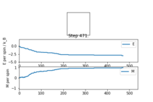
  Figure 53: 8x8 E=1

• 

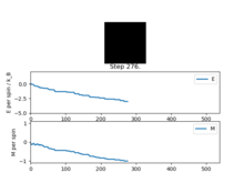
  Figure 54: 8x8 E=-1

• 

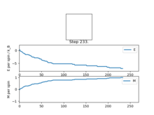
  Figure 55: 8x8 E=5

• 

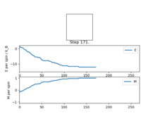
  Figure 56: 8x8 E=10

In the figures above we can see that by varying the electric field we are able to determine which way the lattice chooses to align as the minimum energy conformation will be when all the spins are aligned with one another and also aligned with the electric field. We can also see the effects of increasing the strength of the electric field decreases the time it takes in order for the lattice to reach equilibrium. I would of liked to take this extension further to see how the effects of an electric field vary the curie temperature but due to time constraints this was not possible

Magnetic susceptibility

Magnetic susceptibility can be described as the sensitivity of the average magnetisation to changes in the external field as a fixed temperature. Similar to the relationship between the specific heat capacity and the variance of the total energy is the relationship between the magnetic susceptibility and the variance of the total magnetisation given through,

Thus we can now use our values to plot the magnetic susceptibility as a function of temperature.

We can see that for all the lattice sizes follow the general trend that they are not susceptible to becoming magnetised in an external magnetic field as they are all aligned with one another and so already magnetised. Once we increase the temperature up to the Curie temperature we can see a sudden jump where as this point the spins are trying to achieve maximum entropy and thus loosing their net magnetic dipole and so now the material is susceptible to being magnetised via an external magnetic field. As the temperature is increased to even higher temperatures the thermal energy is higher and thus more and more flipped are being allowed thus it will be harder to magnetise the material and hence the magnetic susceptibility decreases. We can also see that for increasing system sizes the magnetic susceptibility decreases and this can be explained as having a smaller system there are less spins that would need to be flipped to create a magnetised material.