Rep:Bc1015 liquidsimulations

Molecular dynamics simulations of simple liquids

Overall: Nice interpretations on the whole and well written report. Need to get into the style of writing research for your MSci/BSc proj - in computational chemistry if you haven't invented the technicality, don't talk about it in too much depth. The purpose of this lab was more to calculate the diffusive and dynamic properties of phase and you can tie this into other research i.e if you're talking combustion engines, describe how higher diffusion coefficients affect combustion engines. Set an audience for your work! It's particularly important at Imperial because we're so industrially biased :) Mark: 72/100

Report

Abstract

Not a bad abstract - I would put some data into it.

This experiment gave an introduction to the vast potential computer simulations have in research and how simulations can be used to calculate both structural and dynamic properties of different phases. Using a combination of LAMMPS and VMD software allowed the determination of the diffusion coefficient (D) and an accurate picture of how it changes from phase to phase. D increased going from solid to gas, as it is a measure of displacement per unit time for the atoms in the given phase. Our simulations showed that when density is plotted against temperature at a specific pressure, density decreases with time as the system behaves in a more ideal way. Further investigations were carried out, such as how the heat capacity decreases with increasing temperature, or the effect that lattice type has on the heat capacity. The radial distribution function was used to characterise the structures of the systems of our simulations. These results provide understanding on the behaviour of the different phases and the microscopic changes that take place during phase transitions. This has many applications in our day to day.Last sentence is a little vague - if you know an application, put it in!

Introduction

Computer simulations were used to investigate structural and dynamical properties of solids, liquids and gases and the phase transitions between them. Simulations provide a fast and accurate way to gain understanding on how microscopic properties of the system can affect macroscopic parameters, and the results obtained computationally can then be compared to those obtained experimentally to see if they match or to evaluate certain aspects that are difficult to investigate in a lab. Phase changes are constantly occurring around us everyday, gram, don't need this comma from boiling water during cooking, to the phase changes ocurring in an air freshener to allow the prolongation of a scented room. Gaining further understanding of how these phase changes occur has important applications. For example, in this experiment it was studied how heat capacity changes from one phase to another. This can provide insight on how to produce better thermal energy storage systems in buildings and industry to minimise energy waste. Similarly, studies by Thai climate have demonstrated that using phase change materials (PCM) can improve cooling efficiency of air-conditioners. Good intro! Presented your niche.

Aims and Objectives

The aim of this experiment was to be presented to the state-of-art software used in computer simulations, gain a deeper understanding of phase changes and the microscopic and dynamical behaviour in each of the phases and gain insight to the wide range of possibilities when studying a system that computer simulations can provide.This should be less about what you learnt and more about what you calculated - we calculated the dynamics and diffusive properties of phase. Good to know what you learnt though!

Methods

Only include useful information - a good structure for computational methods is *Model*-*Parameters*-*Forcefield*-*Parameters*. The purpose of the methods section isn't to copy out the lab script and going onto MSci/BSc project you need to ensure you're writing like a scientist, not a student :) All simulations were run with the LAMMPS software package. A script was used to define the simulation properties and parameters.Don't need to say this - input scripts are a given for any MD simulation! In the case of liquids and gases the lattice type defined was a simple cubic lattice whereas for solids it was a face centered cubic lattice. The purpose of this rather than starting with random starting coordinates is to set a specific distance between the atoms to prevent them from overlapping which would make the simulation blow up.is this really the purpose of a unit cell structure? If the simulation is run for enough time the atoms will rearrange themselves to more realistic configurations.i.e equilibration The Lennard Jones potential is gram, was - The Lennard Jones is certainly not use in all simulations! used in all simulations to model pair interactions , where there is only one type of atoms of mass 1.0 and the value of both the $\sigma$ and $ϵ$ coefficients is set to one. This script was modified throughout the different parts of the experiment. Dimensionless reduced units were used throughout the whole experiment to make values more manageable.

An initial investigation was carried out to decide what the best timestep to use in our simulations was. The timestep in the script was changed to 0.001, 0.0025, 0.0075, 0.01, 0.015 and the simulation run. VMD software was then used to visualise the trajectories.

The simulations were then modified to run under Npt conditions instead of under NVE (the microcanonical ensemble). The pressures used were $p^{*}$: 1.8 and 2.7 and the temperatures $T^{*}$: 2, 4, 6, 8, and 10. The timestep used was 0.0025, determined to be the best option from the previous experiment.

A script was written to be able to investigate the heat capacity variations between different phases as a function of temperature. The lattice was melted under NVE conditions, and once the melting was finished the system was put under NVT conditions. This enabled us to study the magnitude of the energy fluctuations when the temperature was held constant, which gives us a measure of the heat capacity of the system.

The structures of the systems of our simulations can be characterised using the radial distribution function (RDF), since it gives us an idea of the distances between a reference atom and its nearest neighbours. The RDF for the three phases was calculated using the VMD software mentioned above by setting the selection 1, and 2 to ‘all’, and delta r to 0.05.The density and temperature were modified to give the desired phase. The values were chosen by looking at a Lennard Jones plot.

• Solid: Temperature=1 Density=1.2, and the lattice type was changed from sc to fcc
• Liquid: Temperature=1 Density=0.8
• Gas: Temperature=1 Density=0.02

This software also enabled the calculation of the integrated RDF.

The dynamical properties of the phases can be determined by calculating the diffusion coefficient, which gives a measure of the displacement per unit time for the atoms in each phase. These were calculated by using the mean square displacement (MSD) and velocity autocorrelation function (VACF) plots obtained from our simulations. The results obtained were then compared to those obtained when one million atoms were simulated for each of the phases. This provided a more accurate evaluation on how the diffusion coefficient changes with each phase.

A further investigation was carried out to see how the lattice type affected the heat capacity obtained. The sc lattice type in the script was changed to fcc and hcp and the experiment carried out before was repeated using these new conditions.

Results and Discussion

It is important to ensure that the system reaches an equilibrium state - this is observed when the average values of our thermodynamic quantities become constant. The results obtained from our first experiment when the 0.001 timestep was used show that in the case of our simulation the system did reach equilibrium as can be seen in the graphs below by the energy temperature and pressure reaching a constant value:

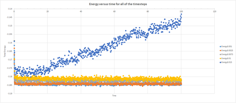
A plot was done showing the energy as a function of time for all timesteps. A compromise has to be done when deciding which timestep to run a simulation with, since greater timesteps take less time to run but you lose information of how the total energy changes in smaller periods of time. The total energy reached equilibrium with all timesteps except 0.015, which instead diverges. Ideally, we want our timestep to give the lowest energy possible, since this defines the most stable configuration. The best timestep was determined to be 0.0025, since it gave the same accuracy as the 0.001 timestep but, since it is larger, it will run faster and may be more suitable for simulations that require observation over a long time.tick

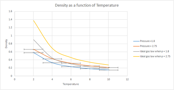
Using this timestep, the script was then modified to run under NpT conditions. The results were plotted using the 2 pressures and the range of temperatures mentioned above. The densities obtained were lower with the lower pressure hate to be obvious but why? Be explicit about every minor detail!. The standard error was slightly greater for the higher pressure. When plotted against the density predicted by the ideal law, it could be seen that at higher temperatures the results obtained from our simulation became more similar to those predicted by the ideal gas law. The simulated density was lower than the one predicted by the ideal gas law. These results can be explained by taking into consideration that in our simulation we are using the Lennard Jones potential to model our pair potential. This model takes into account that the repulsive term dominates at smaller distances and the attractive term at greater distances, whereas in the ideal gas it is assumed that there are no interactions between molecules. Since there is no repulsion between atoms this means than they can get closer to each other, hence resulting in a higher density for the ideal situation.tick As temperature increases, the atoms in our simulation have more energy to move further apart from each other, and hence reducing the interaction between the atoms as the distance between them increases. This situation resembles the ideal gas better, hence we would expect the two plots to overlap at sufficiently high temperatures. The greater the pressure, the larger the deviation from ideality since the atoms are closer together so the interactions are greater. Since the number of atoms in a given volume will be greater because of this, the density is expected to be greater than when smaller pressures are used. tick

Plots obtained when using the pressures 1.8 and 2.7.

Heat capacity is a measure of how much energy is required to raise the temperature by a specific amount. It can be calculated using the following formula:

$C_V=N^2\frac{⟨E^2⟩-{⟨E⟩}^2}{k_B{T}^2}$

To understand better this formula we are going to look at how each part of the equation affects the heat capacity.

N= the greater the number of energy levels populated, the more energy is needed to raise the electron to higher energy levels. This is why hot things (more energy levels populated) are harder to heat up than cold things. Ok but the scaling with N^2 is more the fact that you have more energy levels and thus needs more energy to raise the T
Variance in energy term = it is a measure of the spread of energy levels and how easy it is to populate high energy levels.tick
T= temperature is on the bottom because at high temperature less energy is needed to raise the temperature of the material. but this contradicts your "hot things are harder to heat"? The missing factor is the density of states :)

Another factor to consider is the density of states. If the density of states is higher, it is easier for the higher states to become populated for a given temperature, therefore less energy is required to promote particles to higher energy levels so the heat capacity is lower.

The script used for this simulation is provided below.

After the simulation was run and the results plotted you don't need to say things like this! Just state your observations from your data (make a report more concise) , it was seen that the heat capacity obtained was greater when the larger density was used. A greater density means a greater number of atoms for a given volume, so a greater energy would be required to provide the same amount of energy to all atoms at a specific temperature. At this density, the trend seen was that the heat capacity decreased as temperature increases. At lower density this trend was less pronounced, but as temperature is further increased the same pattern should be obtained due to the density of states - as the temperature increases, the density of states increases as the spacing between energy levels decreases, hence decreasing the heat capacity as less energy is required to promote atoms to higher energy levels. However, as temperature increases more degrees of freedom become accessible by the equipartition theorem, therefore this might potentially increase the heat capacity instead. The final result will be a compromise between these two competing processes.tick

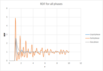
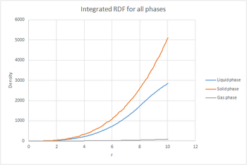
The radial distribution function, $g(r)$ was calculated. An analogy can be made between the radial distribution function and the wavefunction, in the sense that neither of them have a physical meaning on its own. This is why we also calculate $\int g(r)\mathrm{d}r$, as this gives us an idea of Doesn't just give us an idea of! the density of the system and gives us a way to calculate the number of particles in each coordination shell. The RDFs were plotted as a function of distance (r). The gas plot has an initial large peak and then levels off levels off is too colloquial. This suggests that there is single diffuse coordination sphere. The liquid also has the initial peak but then has smaller oscillations until it finally levels off. This greater number of peaks suggests a greater number of coordination spheres than in a gas. The RDF for the solid is much more complex - there is gram, are a greater number of sharp peaks reflecting the crystal structure of the solid. The peaks are sharp compared to the broad peaks in the liquid because in a solid the particles are fixed in place whereas in a liquid they are held less tightly so they can spread out across the coordination shell.Dynamic averaging Since the peaks represent distinct spheres of coordination, the troughs must represent the areas between the shells.

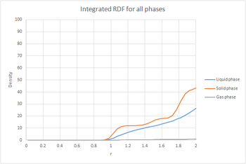
The plots of the integrated RDF are simpler, the general trend being that in the three cases the density increased in an exponential manner with increasing r.

By considering that $g(r)\mathrm{d}r$ is a measure of density, the plot of the solid can be used to determine the coordination number for each of the first three peaks. The first peak has a value of approxinately 12, the second around 18 and the third around 42. This would mean that the number of nearest neighbours in the first peak is 12, in the second 8 and in the third 24 since it is cumulative. These values match the expected values for a fcc lattice. Looking at the log file for the solid, the lattice spacing was calculated to be 1.4938.tick

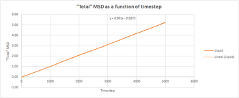
The total MSD was plotted as a function of time for the three phases for both our simulation and the one million atom simulations. Both the trend and the shape of the graphs were the same in both cases. The solid phase has an initial spike but then oscillates around a average value, which was used to take a trendline to be able to determine the diffusion coefficient.This oscillations could be due to the system reaching equilibrium. The liquid follows a linear trend from the beginning since there is no ballistic region. A trendline was also determined and the gradient calculated. With the gas phase there is an initial ballistic region and then a linear region when diffusion is taking place. The gradient was determined solely using this linear part.tick

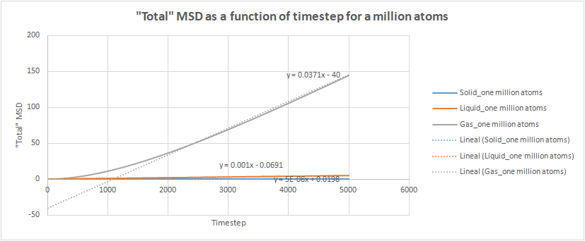
Once the gradient was calculated, the diffusion coefficient was determined using the following equation. Since the units of the diffusion coefficient are $m^2{s}^{-1}$, the formula had to include a term to convert from timestep (0.0025 used) to seconds:

$D=\frac{1}{6}\frac{1}{timestep}\frac{\partial ⟨r^2\left(t\right)⟩}{\partial t}$

Where the term $\frac{\partial ⟨r^2\left(t\right)⟩}{\partial t}$ is the gradient of our plot.

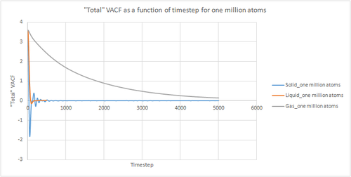
The VACF gives us a measure of how the velocity can change over time. The oscillations in VACF give us an idea of the collisions taking place since collisions change the diffusive properties of atoms as the collision are unlikely to be completely elastic.tick All graphs start at a maximum since at the beinninggram the atom has a specific velocity, and then decay since during short time periods there will be a degree of correlation between the velocity of the atom and its velocity a short time in the past. If the atoms in the system did not interact with each other, the Newton's Laws of motion tell us that the atom would retain this maximum velocity for all time, but this is not the case in real systems. The peaks just correspond to collisions like the first minimum is the point at which the particles have all collided at least once e.t.c

In the case of both liquids and solids the atoms are close together and hence experience interatomic interactions. The atoms will therefore seek to find the most stable location which will be a compromise between the repulsive and attractive forces. For a solid, we see a damped harmonic motion since it is the most dense system, the atoms are closer together and hence the interatomic interactions are stronger. hmm I wouldn't say it's DHM.. there are too many collisions for it! The atoms will oscillate backwards and forwards due to the competing repulsive and attractive forces. Each time the motion is reversed, the velocity changes sign as we can see in the plot. The minima in the graph therefore represent the point of maximum displacement between the atoms before the velocity is reversed. Since the collisions are non elastic the magnitude of the oscillations decreases with time. At $C\left(\mathrm{\infty }\right)=0$ as the velocities of atoms should become uncorrelated with time.

Liquids have a similar shape but since the atoms are further apart the interatomic forces are weaker and hence less oscillations are observed.

In gases, the atoms are much further apart and hence the interatomic forces are weaker. It will hence take longer for the velocity to become uncorrelated as less collisions occur per unit time compared to liquids and solids. true.

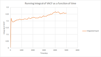
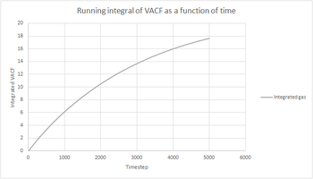
The trapezium rule was used to approximate the integral under the VACF for all phases of both our simulations and the one million atoms simulations. It is an approximation since the tops of the trapezia will not exactly match the shape of the curve. This will introduce a degree of error in the results obtained and will be the largest source of error in the estimates of D from the VACF. To increase the accuracy, more and thinner strips could be used in the approximation, but this would probably make the calculation more cumbersome. The shapes of the graphs obtained were the same for our simulations and the one million atoms simulations.trapezium rule does provide an extra element of inaccuracy with bin widths..

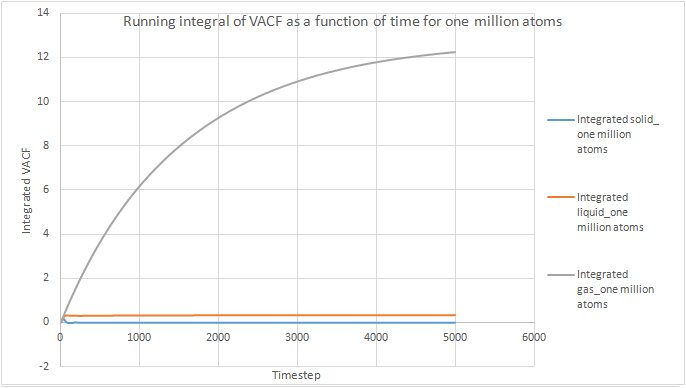
The running integral can be used to estimate the value of the diffusion coefficient by the following formula:

$D=\frac{1}{3}\underset{0}{\overset{\mathrm{\infty }}{\int }}\mathrm{d}\tau ⟨\mathbf{v}\left(0\right)\cdot \mathbf{v}\left(\tau \right)⟩$

Where the term $\underset{0}{\overset{\mathrm{\infty }}{\int }}\mathrm{d}\tau ⟨\mathbf{v}\left(0\right)\cdot \mathbf{v}\left(\tau \right)⟩$ is the running integral.

The calculated diffusion coefficients are given below:

Diffusion coefficients obtained (m²s^-1)

Phase	MSD own simulations	MSD one million atoms	VACF own simulations	VACF one million atoms
Solid	3.33E-07	3.33E-06	-1.47E-04	5.70E-05
Liquid	6.67E-02	6.67E-02	8.62E-02	1.13E-01
Gas	4.85E+00	2.47E+00	5.88E+00	4.09E+00

tick

We would expect the values obtained for the one million atoms to be more reliable. This is because the greater the number of atoms used to calculate the total MSD or VACF, the more accurate the value. The diffusion coefficient is a measure of the displacement per unit time, so the results match the expected values - the denser the substance the more difficult for the atoms to move so we would expect the solid to have the lowest diffusion coefficient, which is what we see . Our value of D is so small that this suggests there is practically no diffusion in solids. The diffusion coefficients obtained for the VACF are of approximately the same magnitude as those obtained from the MSD, making our results more reliable.tick

The heat capacity experiment was repeated but changing the type of lattice in the simulation. A sc unit cell contains one single atom, whereas a fcc unit cell contains 4 atoms and an hcp unit cell contains 6 atoms. One would expect that as the number of atoms in the unit cell increases, more energy is required for a given temperature to be able to heat all atoms to the same extent and hence a higher heat capacity would be expected.tick, nice

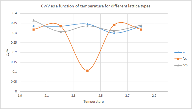
However, when the results were plotted, no apparent trend was observed. The shape of the fcc plot was unexpected. A possible suggestion for the large minimum could be a change of phase, however, further investigation would be required to fully understand the reasoning behind the shape of this graph.but were the absolute magnitudes for the systems of the same properties different?

Conclusion

It's always nice to tie conclusions back to intro which you have done with your ultimate description of this work being a general overview of MD. Would have been nice for the goal to be scientific rather than technical but not bad. It's good to talk about your important data/possible errors/future work in your conclusion. We work in a quantitative world! But not bad! The best timestep determined was 0.0025, as it was the largest timestep to give accurate results. This was then used in all other experiments. Running the simulation under NpT conditions and comparing against the results obtained using the ideal gas law demonstrated that as temperature increases the simulations are expected to behave in a more ideal manner as the interactions between the atoms are minimised as temperature increases because the distance between the atoms increases. When the simulations were run at a greater pressure the results deviated more from ideality because as the atoms are closer together the interactions are stronger so it behaves less ideally. This also means that the density will be greater than if a smaller pressure is used as the atoms are expected to be found closer together.

The heat capacity was greater when a greater density was used and the trend observed was that the heat capacity decreased with increasing temperature. The main explanation behind this is taking into account the density of states, because if the temperature increases the density of states is greater so less energy is required for promotion to higher energy levels so the heat capacity is lower. A greater density means a greater number of atoms per given volume so more energy is required to get each atom to the same temperature, so the heat capacity is greater.tick, good

The integrated RDF allows us to characterise the structures of the systems of our simulations and to gain insight of the coordination shells in each of the phases. The results obtained for the coordination number in a solid match those expected for a face centered cubic lattice.

The diffusion coefficient for each of the phases was determined using the MSD and VACF plots, the solid having a negligible diffusion coefficient and D increasing as the phase becomes less dense, as D is a measure of displacement per unit time. The one million atoms simulations provided more accurate results as the greater number of atoms meant a more reliable average was obtained.

The results from the investigation of how lattice type affects heat capacity were inconclusive, and further investigation would be required to fully understand the shape of the graph.

Overall, LAMMPS software provided an effective way to allow us to simulate the behaviour of the three phases to investigate and calculate different structural and dynamical properties of solids, liquids and gases and gain further insight of the phase transitions between these. The Lennard Jones potential proved to be a good model for these simulations. This field is important since phase transitions occur all around us everyday, and having a better understanding on the microscopic changes during the phase transitions can provide better solutions in many applications.tick

Tasks

Introduction to molecular dynamics simulation

Numerical Integration

TASK: Open the file HO.xls. In it, the velocity-Verlet algorithm is used to model the behaviour of a classical harmonic oscillator. Complete the three columns "ANALYTICAL", "ERROR", and "ENERGY": "ANALYTICAL" should contain the value of the classical solution for the position at time t, "ERROR" should contain the absolute difference between "ANALYTICAL" and the velocity-Verlet solution (i.e. ERROR should always be positive -- make sure you leave the half step rows blank!), and "ENERGY" should contain the total energy of the oscillator for the velocity-Verlet solution. Remember that the position of a classical harmonic oscillator is given by $x\left(t\right)=A\cos (\omega t+\varphi )$ (the values of A, $\omega$, and $\varphi$ are worked out for you in the sheet).

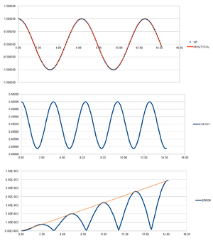
The given equation was used to calculate the position at time T. To ensure that ERROR was always positive, the function ABS was used in excel, and the difference between the "ANALYTICAL" and the velocity-Verlet solution was calculated. The total energy of the oscillator was determined by adding the potential energy ($\frac{1}{2}k{x}^2)$ and the kinetic energy ($\frac{1}{2}m{v}^2$ ). The following graphs were obtained:

Image showing the three graphs produced after completing the analytical, error and energy columns for a timestep of 0.1.

TASK: For the default timestep value, 0.1, estimate the positions of the maxima in the ERROR column as a function of time. Make a plot showing these values as a function of time, and fit an appropriate function to the data.

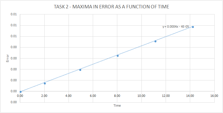
The following graph was obtained when the position of the maxima in the ERROR column were estimated. The points followed a linear relationship, making it possible for a trendline to be plotted. The equation of this trendline was y = 0.0004x - 4E-05.

TASK: Experiment with different values of the timestep. What sort of a timestep do you need to use to ensure that the total energy does not change by more than 1% over the course of your "simulation"? Why do you think it is important to monitor the total energy of a physical system when modelling its behaviour numerically?

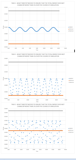
A formula was created to be able to determine 1% from the maximum value in Energy and then adding and subtracting this to find the minimum and maximum values to ensure that the total energy didn't change by more than 1% over the course of the simulation. After trying different values for the timestep, it was seen that the maximum value that didn't result in the total energy of the simulation going below the minimum line was when the timestep was 0.2. It is important to monitor the total energy of a physical system when modelling its behaviour numerically because this will affect the accuracy of calculations. Monitoring the total energy of a system is also important because it is a way to help us understand what is happening in the physical system.

Image showing the three graphs obtained when the timestep was changed. The first corresponds to the 0.1 timestep, and the other two for the 0.2 and 0.3 respectively.

Atomic Forces

TASK: For a single Lennard-Jones interaction, $\varphi \left(r\right)=4ϵ(\frac{{\sigma }^{12}}{r^{12}}-\frac{{\sigma }^6}{r^6})$, find the separation, $r_0$, at which the potential energy is zero. What is the force at this separation? Find the equilibrium separation, $r_{eq}$, and work out the well depth ($\varphi \left(r_{eq}\right)$). Evaluate the integrals $\underset{2\sigma }{\overset{\mathrm{\infty }}{\int }}\varphi \left(r\right)\mathrm{d}r$, $\underset{2.5\sigma }{\overset{\mathrm{\infty }}{\int }}\varphi \left(r\right)\mathrm{d}r$, and $\underset{3\sigma }{\overset{\mathrm{\infty }}{\int }}\varphi \left(r\right)\mathrm{d}r$ when $\sigma =ϵ=1.0$.

$0=4ϵ(\frac{{\sigma }^{12}}{r^{12}}-\frac{{\sigma }^6}{r^6})$

$0=(\frac{{\sigma }^{12}}{r^{12}}-\frac{{\sigma }^6}{r^6})$

$\frac{{\sigma }^{12}}{r^{12}}=\frac{{\sigma }^6}{r^6}$

${\sigma }^6=r^6$

$r_0=\sigma$

To find the force at this separation, we have to find the derivative of the potential, since $F=-\frac{dU(r^N)}{d{r}_i}$.
$U=4ϵ({\sigma }^{12}{r}^{-12}-{\sigma }^6{r}^{-6})$

$F=-4ϵ(-12{\sigma }^{12}{r}^{-13}+6{\sigma }^6{r}^{-7})$

Since $r=\sigma$ this equation then becomes:

$F=-4ϵ(\frac{-12{\sigma }^{12}}{{\sigma }^{13}}+\frac{6{\sigma }^6}{{\sigma }^7})$

$F=-4ϵ(\frac{-12}{\sigma }+\frac{6}{\sigma })$

$F=-4ϵ(\frac{-6}{\sigma })$

$F=\frac{24ϵ}{\sigma }$

At equilibrium, there are no net forces so the derivative becomes 0.
$0=-4ϵ(\frac{-12{\sigma }^{12}}{r^{13}}+\frac{6{\sigma }^6}{r^7})$

$0=(\frac{-12{\sigma }^{12}}{r^{13}}+\frac{6{\sigma }^6}{r^7})$

$0=\frac{6{\sigma }^6}{r^7}(\frac{-2{\sigma }^6}{r^6}+1)$

$1=\frac{2{\sigma }^6}{r^6}$

$r^6=2{\sigma }^6$

$r_{eq}=2^{\frac{1}{6}}\sigma$

The well depth is the value for the minimum value for the potential in the Lennard Jones curve, that is, the value of the potential when the system is at equilibrium. Using the result shown above:
$U=4ϵ(\frac{{\sigma }^{12}}{(2^{\frac{1}{6}}\sigma {)}^{12}}-\frac{{\sigma }^6}{(2^{\frac{1}{6}}\sigma {)}^6})$

$U=4ϵ(\frac{1}{2^{\frac{12}{6}}}-\frac{1}{2^{\frac{6}{6}}})$

$U=4ϵ(\frac{1}{2^2}-\frac{1}{2})$

$U=4ϵ(-\frac{1}{4})$

$U=-ϵ$

Evaluating the integrals when $\sigma =ϵ=1.0$:
$U=4ϵ({\sigma }^{12}{r}^{-12}-{\sigma }^6{r}^{-6})$

$\underset{2\sigma }{\overset{\mathrm{\infty }}{\int }}\varphi \left(r\right)\mathrm{d}r=4ϵ(\frac{{\sigma }^{12}{r}^{-11}}{-11}-\frac{{\sigma }^6{r}^{-5}}{-5})$

$\underset{2\sigma }{\overset{\mathrm{\infty }}{\int }}\varphi \left(r\right)\mathrm{d}r=4ϵ(\frac{-{\sigma }^{12}}{11r^{11}}+\frac{{\sigma }^6}{5r^5})$

$\underset{2\sigma }{\overset{\mathrm{\infty }}{\int }}\varphi \left(r\right)\mathrm{d}r=4(\frac{-1}{11(2^{11})}+\frac{1}{5(2^5)})$

$\underset{2\sigma }{\overset{\mathrm{\infty }}{\int }}\varphi \left(r\right)\mathrm{d}r=-0.0248$

$\underset{2.5\sigma }{\overset{\mathrm{\infty }}{\int }}\varphi \left(r\right)\mathrm{d}r=-0.00818$

$\underset{3\sigma }{\overset{\mathrm{\infty }}{\int }}\varphi \left(r\right)\mathrm{d}r=-0.00329$

TASK: Estimate the number of water molecules in 1ml of water under standard conditions. Estimate the volume of 10000 water molecules under standard conditions.

The standard state of water is pure water, which has a concentration of 55.5M.

The number of molecules in 1ml of water can be calculated with the following formula:

number of molecules = number of moles x Avogadro's constant (6.02x10²³)

number of molecules = concentration x volume x Avogadro's constant (6.02x10²³)

number of molecules = 1x10^-3 L x 55.5 M x 6.02x10²³

number of molecules = 3.34x10²²

This same equation can also be used to determine the volume of 10000 water molecules.

1000 = volume x 55.5 M x 6.02x10²³

volume = 2.99x10^-23 L

TASK: Consider an atom at position $(0.5,0.5,0.5)$ in a cubic simulation box which runs from $(0,0,0)$ to $(1,1,1)$. In a single timestep, it moves along the vector $(0.7,0.6,0.2)$. At what point does it end up, after the periodic boundary conditions have been applied?.

The atom will finish at $(0.2,0.1,0.7)$ after the periodic boundary conditions are applied.

Reduced Units

TASK: The Lennard-Jones parameters for argon are $\sigma =0.34\mathrm{n}\mathrm{m}$, $$\begin{gathered} ϵ \\ / \\ {k}_B=120\mathrm{K} \end{gathered}$$. If the LJ cutoff is $r^{*}=3.2$, what is it in real units? What is the well depth in $$\begin{gathered} {\mathrm{k}\mathrm{J} \\ \mathrm{m}\mathrm{o}\mathrm{l}}^{-1} \end{gathered}$$? What is the reduced temperature $T^{*}=1.5$ in real units?

The reduced units are calculated using the following equations:
distance $r^{*}=\frac{r}{\sigma }$
energy $E^{*}=\frac{E}{ϵ}$
temperature $T^{*}=\frac{k_{B}T}{ϵ}$
Reduced units are used to make the values dimensionless and more manageable.

The first equation can be used to determine LJ cutoff in real units. Multiplying $r^{*}=3.2$ by $\sigma =0.34\mathrm{n}\mathrm{m}$, we determine that $r=1.09nm$.

It was shown above that the potential well depth is $-ϵ$, hence:

$-ϵ=-120K.k_B$ where $k_B=1.38x10^{-23}J{K}^{-1}$
$-ϵ=-1.66x10^{-21}J$

To get $mo{l}^{-1}$ in the units multiply times Avogadro's constant:

$-ϵ=966.9J{K}^{-1}mo{l}^{-1}=-0.966kJmo{l}^{-1}$

Rearranging the equation for the reduced temperature:

temperature $T=\frac{ϵ.T^{*}}{k_B}$
And we know that: $\frac{ϵ}{k_B}=120K$
temperature $T=120Kx1.5$
temperature $T=180K$

Equilibration

Creating the simulation box

TASK: Why do you think giving atoms random starting coordinates causes problems in simulations? Hint: what happens if two atoms happen to be generated close together?

The simulation will "blow up" if two particles overlap. We avoid this from happening by assigning the atoms to vertices of a lattice, hence setting a determined distance between the atoms to avoid the overlap.

TASK: Satisfy yourself that this lattice spacing corresponds to a number density of lattice points of 0.8. Consider instead a face-centred cubic lattice with a lattice point number density of 1.2. What is the side length of the cubic unit cell?

A simple cubic lattice has a single atom per unit cell. From the log file we know that the lattice spacing is 1.07722, therefore:
$numberdensity=\frac{1}{l^3}$
$numberdensity=\frac{1}{(1.07722{)}^3}$
$numberdensity=0.8(1d.p.)$

A face centred cubic lattice contains 4 atoms, therefore:
$numberdensity=\frac{4}{l^3}$
$l=\sqrt[3]{(}\frac{4}{1.2})=1.4938$

TASK: Consider again the face-centred cubic lattice from the previous task. How many atoms would be created by the create_atoms command if you had defined that lattice instead?

The box we have defined contains 1000 (10x10x10) unit cells. Since for a face centred cubic lattice there are 4 atoms per unit cell, there would be 4000 atoms created by the command.

Setting the properties of the atoms

TASK: Using the LAMMPS manual, find the purpose of the following commands in the input script:

mass 1 1.0
pair_style lj/cut 3.0
pair_coeff * * 1.0 1.0

The first command sets the mass for all atoms of one or more atom types. It means that for atom of type 1 the mass is 1.0. The second command sets the formula(s) LAMMPS uses to compute pairwise interactions. In LAMMPS, pair potentials are defined between pairs of atoms that are within a cutoff distance and the set of active interactions typically changes over time. In our case s the Lennard-Jones potential is used to model the pair potential and the cuttoff distance is 3.0. The pair_coeff command specifies the pairwise force field coefficients for one or more pairs of atom types, where the asterisks correspond to the atom types, and the two following 1.0 are $\sigma$ and $ϵ$ respectively.

TASK: Given that we are specifying ${\mathbf{x}}_i\left(0\right)$ and ${\mathbf{v}}_i\left(0\right)$, which integration algorithm are we going to use?

We will be using the Velocity Verlet algorithm since we are defining the starting position of the atom and the velocity at the same time.

Running the simulation

TASK: Look at the lines below.

SPECIFY TIMESTEP
variable timestep equal 0.001
variable n_steps equal floor(100/${timestep})
timestep ${timestep}

RUN SIMULATION
run ${n_steps}
run 100000

The second line (starting "variable timestep...") tells LAMMPS that if it encounters the text ${timestep} on a subsequent line, it should replace it by the value given. In this case, the value ${timestep} is always replaced by 0.001. In light of this, what do you think the purpose of these lines is? Why not just write:

timestep 0.001
run 100000
Ask the demonstrator if you need help.

The first code is preferred because in this case the timestep is defined as a variable. We can change the value of the timestep simply by changing the value in that line and we can then call the variable at any point in the code using ${timestep} instead of having to repeatedly define it again throughout the code.

Checking equilibration

TASK: make plots of the energy, temperature, and pressure, against time for the 0.001 timestep experiment (attach a picture to your report). Does the simulation reach equilibrium? How long does this take? When you have done this, make a single plot which shows the energy versus time for all of the timesteps (again, attach a picture to your report). Choosing a timestep is a balancing act: the shorter the timestep, the more accurately the results of your simulation will reflect the physical reality; short timesteps, however, mean that the same number of simulation steps cover a shorter amount of actual time, and this is very unhelpful if the process you want to study requires observation over a long time. Of the five timesteps that you used, which is the largest to give acceptable results? Which one of the five is a particularly bad choice? Why?

When the simulation was run with the 0.001 timestep equilibration was reached very quickly (within the first four timesteps), seen by the energy temperature and pressure reaching a constant value.

A plot was done showing the energy as a function of time for all timesteps. A compromise has to be done when deciding which timestep to run a simulation with, since greater timesteps take less time to run but you lose information of how the total energy changes in smaller periods of time. This is why for the 0.015 timestep the total energy diverges over time, and hence is a particularly bad choice since we expect the plots to converge. The best timestep was determined to be 0.0025, since it gave the same accuracy as the 0.001 timestep but, since it is larger, it will run faster and may be more suitable for simulations that require observation over a long time.

Running simulations under specific conditions

Temperature and Pressure Control

TASK: Choose 5 temperatures (above the critical temperature T^* = 1.5), and two pressures (you can get a good idea of what a reasonable pressure is in Lennard-Jones units by looking at the average pressure of your simulations from the last section). This gives ten phase points — five temperatures at each pressure. Create 10 copies of npt.in, and modify each to run a simulation at one of your chosen \left(p, T\right) points. You should be able to use the results of the previous section to choose a timestep. Submit these ten jobs to the HPC portal. While you wait for them to finish, you should read the next section.

The pressures chosen where 2.5 and 2.7 since these were within the range of values when the pressure averaged in the equilibration section, and the temperatures were 2,2.5,3,3.5 and 5. The timestep used was 0.0025, as it was determined before that it was the largest to give acceptable results.

Thermostats and Barostats

TASK: We need to choose $\gamma$ so that the temperature is correct $T=\mathfrak{𝔗}$ if we multiply every velocity $\gamma$. We can write two equations:

$\frac{1}{2}\sum _i{m}_i{v}_i^2=\frac{3}{2}N{k}_{B}T$

$\frac{1}{2}\sum _i{m}_i{\left(\gamma v_i\right)}^2=\frac{3}{2}N{k}_B\mathfrak{𝔗}$

Solve these to determine $\gamma$.

To solve these we shall divide one equation by the other:

$\frac{\frac{1}{2}\sum _i{m}_i{\left(\gamma v_i\right)}^2}{\frac{1}{2}\sum _i{v}_i^2}=\frac{\frac{3}{2}N{k}_B\mathfrak{𝔗}}{\frac{3}{2}N{k}_{B}T}$
By doing this, most of the values cancel out, simplifying the equation to the following form:
$\frac{\sum _i{\left(\gamma v_i\right)}^2}{\sum _i{v}_i^2}=\frac{\mathfrak{𝔗}}{T}$
We can now solve for $\gamma$:
$\frac{\sum _i{\gamma }^2{v}_i^2}{\sum _i{v}_i^2}=\frac{\mathfrak{𝔗}}{T}$
$\frac{{\gamma }^2\sum _i{v}_i^2}{\sum _i{v}_i^2}=\frac{\mathfrak{𝔗}}{T}$
${\gamma }^2=\frac{\mathfrak{𝔗}}{T}$
$\gamma =\sqrt{\frac{\mathfrak{𝔗}}{T}}$
This means that when $T=\mathfrak{𝔗}$:
$\gamma =1$

Examining the Input Script

TASK: Use the manual page to find out the importance of the three numbers 100 1000 100000. How often will values of the temperature, etc., be sampled for the average? How many measurements contribute to the average? Looking to the following line, how much time will you simulate?

The numbers correspond to:
100=N_every - use input values every this many timesteps
1000=N_repeat - # of times to use input values for calculating averages
100000=N_freq - calculate averages every this many timesteps

The first number means that an average is taken every 100 values. N_repeat determines how many of those averages are used to calculate the overall average. N_freq is a multiple of N_every and N_repeat and determines that an average is taken every 100000 timestep. The time simulated will be 100000 * the timestep. Since the timestep used was 0.0025, 250 s will be simulated.

Plotting the Equations of State

TASK: When your simulations have finished, download the log files as before. At the end of the log file, LAMMPS will output the values and errors for the pressure, temperature, and density $\left(\frac{N}{V}\right)$. Use software of your choice to plot the density as a function of temperature for both of the pressures that you simulated. Your graph(s) should include error bars in both the x and y directions. You should also include a line corresponding to the density predicted by the ideal gas law at that pressure. Is your simulated density lower or higher? Justify this. Does the discrepancy increase or decrease with pressure?

Plots obtained when using the pressures 2.5 and 2.7.

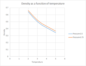
When the results were plotted, the general trend for both pressures was for the density to decrease with increasing temperature. However, as the chosen pressures were very close together the two plots weren't very different, so the simulation was repeated using the pressures=1.8 and 2.7 and using a wider range of temperatures. When these results were plotted a greater difference was observed between the plots. The densities obtained were lower with the lower pressure. The standard error was slightly greater for the higher pressure. When plotted against the density predicted by the ideal law, it could be seen that at higher temperatures the results obtained from our simulation became more similar than those predicted by the ideal gas law. The simulated density was lower than the one predicted by the ideal gas law. Both these results can be explained by taking into consideration that in the Lennard Jones potential the repulsive term dominates whereas in the ideal gas it is assumed that there are no interactions between molecules. Since there is no repulsion between atoms this means than they can get closer to each other, hence resulting in a higher density. As temperature increases, the atoms in our simulation have more energy to move further apart from each other, and hence reducing the interaction between the atoms as the distance between them increases. This situation resembles the ideal gas better, hence we would expect the two plots to overlap at sufficiently high temperatures.

Plots obtained when using the pressures 1.8 and 2.7.

Calculating heat capacities

TASK: As in the last section, you need to run simulations at ten phase points. In this section, we will be in density-temperature $({\rho }^{*},T^{*})$ phase space, rather than pressure-temperature phase space. The two densities required at 0.2 and 0.8, and the temperature range is 2.0, 2.2, 2.4, 2.6, 2.8. Plot $C_V/V$ as a function of temperature, where V is the volume of the simulation cell, for both of your densities (on the same graph). Is the trend the one you would expect? Attach an example of one of your input scripts to your report.

Heat capacity is a measure of how much energy is required to raise the temperature by a specific amount. It can be calculated using the following formula:

$C_V=N^2\frac{⟨E^2⟩-{⟨E⟩}^2}{k_B{T}^2}$

To understand better this formula we are going to look at how each part of the equation affects the heat capacity.

N= the greater the number of energy levels populated, the more energy is needed to raise the electron to higher energy levels. This is why hot things (more energy levels populated) are harder to heat up than cold things.
Variance in energy term = it is a measure of the spread of energy levels and how easy it is to populate high energy levels.
T= temperature is on the bottom because at high temperature less energy is needed to raise the temperature of the material.

Another factor to consider is the density of states. If the density of states is higher, it is easier for the higher states to become populated for a given temperature, therefore less energy is required to excite particles to higher energy levels so the heat capacity is lower.

The script used for this simulation is provided below.

After the simulation was run and the results plotted, it was seen that the heat capacity obtained was greater when the larger density was used. A greater density means a greater number of atoms for a given volume, so a greater energy would be required to provide the same amount of energy to all atoms at a specific temperature. At this density, the trend seen was that the heat capacity decreased as temperature increases. At lower density this trend was less pronounced, but as temperature is further increased the same pattern should be obtained due to the density of states - as the temperature increases, the density of states increases, hence decreasing the heat capacity. However, as temperature increases more degrees of freedom become accessible by the equipartition theorem, therefore this might potentially increase the heat capacity instead. The final result will be a compromise between these two competing processes.

Structural properties and the radial distribution function

TASK: perform simulations of the Lennard-Jones system in the three phases. When each is complete, download the trajectory and calculate $g(r)$ and $\int g(r)\mathrm{d}r$. Plot the RDFs for the three systems on the same axes, and attach a copy to your report. Discuss qualitatively the differences between the three RDFs, and what this tells you about the structure of the system in each phase. In the solid case, illustrate which lattice sites the first three peaks correspond to. What is the lattice spacing? What is the coordination number for each of the first three peaks?

The density and temperature were modified to give the desired phase. The values were chosen by looking at a Lennard Jones plot.

• Solid: Temperature=1 Density=1.2, and the lattice type was changed from sc to fcc
• Liquid: Temperature=1 Density=0.8
• Gas: Temperature=1 Density=0.02

The radial distribution function, $g(r)$ was calculated. An analogy can be made between the radial distribution function and the wavefunction, in the sense that neither of them have a physical meaning on its own. This is why we also calculate $\int g(r)\mathrm{d}r$, as this gives us an idea of the density of the system. The RDFs were plotted as a function of time. The gas plot has an initial large peak and then levels off. The liquid also has the initial peak but then has smaller oscillations until it finally levels off. The RDF for the solid is much more complex. The plots of the integrated RDF are simpler, the general trend being that in the three cases the density increased in an exponential manner with increasing r.

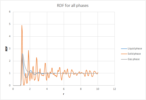
By considering that $g(r)\mathrm{d}r$ is a measure of density, the plot of the solid can be used to determine the coordination number for each of the first three peaks. The first peak has a value of approxinately 12, the second around 18 and the third around 42. This would mean that the number of nearest neighbours in the first peak is 12, in the second 8 and in the third 24 since it is cumulative. These values match the expected values for a fcc lattice. Looking at the log file for the solid, the lattice spacing was calculated to be 1.4938.

Dynamical properties and the diffusion coefficient

Simulations in this Section

TASK: In the D subfolder, there is a file liq.in that will run a simulation at specified density and temperature to calculate the mean squared displacement and velocity autocorrelation function of your system. Run one of these simulations for a vapour, liquid, and solid. You have also been given some simulated data from much larger systems (approximately one million atoms). You will need these files later.

The same values as before were used to simulate the vapour, liquid and solid phases, and the lattice type for the solid was changed from sc to fcc.

Mean Squared Displacement

TASK: make a plot for each of your simulations (solid, liquid, and gas), showing the mean squared displacement (the "total" MSD) as a function of timestep. Are these as you would expect? Estimate D in each case. Be careful with the units! Repeat this procedure for the MSD data that you were given from the one million atom simulations.

The total MSD was plotted as a function of time for the three phases for both our simulation and the one million atom simulations. Both the trend and the shape of the graphs were the same in both cases. The solid phase has an initial spike but then oscillates around a average value, which was used to take a trendline to be able to determine the diffusion coefficient. The liquid follows a linear trend from the beginning since there is no ballistic region. A trendline was also determined and the gradient calculated. With the gas phase there is an initial ballistic region and then a linear region when diffusion is taking place. The gradient was determined solely using this linear part.

Once the gradient was calculated, the diffusion coefficient was determined using the following equation. Since the units of the diffusion coefficient are $m^2{s}^{-1}$, the formula has to include a term to convert from timestep (0.0025 used) to seconds:

$D=\frac{1}{6}\frac{1}{timestep}\frac{\partial ⟨r^2\left(t\right)⟩}{\partial t}$

Where the term $\frac{\partial ⟨r^2\left(t\right)⟩}{\partial t}$ is the gradient of our plot.

The calculated diffusion coefficients are given below:

Diffusion coefficients for our simulations

Phase	Diffusion coefficient (m2s-1)
Solid	3.33E-07
Liquid	6.67E-02
Gas	4.85E+00

Diffusion coefficients for one million atoms simulations

Phase	Diffusion coefficient (m2s-1)
Solid	3.33E-06
Liquid	6.67E-02
Gas	2.47E+00

We would expect the values obtained for the one million atoms to be more reliable. This is because the MSD is an average so the greater the number of atoms used to calculate it, the more accurate the average. The diffusion coefficient is a measure of the displacement per unit time, so the results match the expected values - the denser the substance the more difficult for the atoms to move so we would expect the solid to have the lowest diffusion coefficient.

EXTENSION: Velocity Autocorrelation Function

TASK: In the theoretical section at the beginning, the equation for the evolution of the position of a 1D harmonic oscillator as a function of time was given. Using this, evaluate the normalised velocity autocorrelation function for a 1D harmonic oscillator (it is analytic!):

$C\left(\tau \right)=\frac{\underset{-\mathrm{\infty }}{\overset{\mathrm{\infty }}{\int }}v\left(t\right)v(t+\tau )\mathrm{d}t}{\underset{-\mathrm{\infty }}{\overset{\mathrm{\infty }}{\int }}{v}^2\left(t\right)\mathrm{d}t}$

Be sure to show your working in your writeup. On the same graph, with x range 0 to 500, plot $C\left(\tau \right)$ with $\omega =1/2\pi$ and the VACFs from your liquid and solid simulations. What do the minima in the VACFs for the liquid and solid system represent? Discuss the origin of the differences between the liquid and solid VACFs. The harmonic oscillator VACF is very different to the Lennard Jones solid and liquid. Why is this? Attach a copy of your plot to your writeup.

$C\left(\tau \right)=\frac{\underset{-\mathrm{\infty }}{\overset{\mathrm{\infty }}{\int }}v\left(t\right)v(t+\tau )\mathrm{d}t}{\underset{-\mathrm{\infty }}{\overset{\mathrm{\infty }}{\int }}{v}^2\left(t\right)\mathrm{d}t}$
$x\left(t\right)=A\cos (\omega t+\varphi )$
$v(t)=\frac{dx}{dt}=-A\omega \sin (\omega t+\varphi )$
$C\left(\tau \right)=\frac{\underset{-\mathrm{\infty }}{\overset{\mathrm{\infty }}{\int }}(-A\omega \sin (\omega t+\varphi ))(-A\omega \sin (\omega t+\omega t+\varphi ))\mathrm{d}t}{\underset{-\mathrm{\infty }}{\overset{\mathrm{\infty }}{\int }}{A}^2{\omega }^2{\sin }^2(\omega t+\varphi )\mathrm{d}t}$
$C\left(\tau \right)=\frac{\underset{-\mathrm{\infty }}{\overset{\mathrm{\infty }}{\int }}{A}^2{\omega }^2(\sin (\omega t+\varphi ))(\sin (\omega t+\varphi )\cos (\omega t)+\cos (\omega t+\varphi )\sin (\omega t))\mathrm{d}t}{\underset{-\mathrm{\infty }}{\overset{\mathrm{\infty }}{\int }}{A}^2{\omega }^2{\sin }^2(\omega t+\varphi )\mathrm{d}t}$
$C\left(\tau \right)=\frac{\underset{-\mathrm{\infty }}{\overset{\mathrm{\infty }}{\int }}{\sin }^2(\omega t+\varphi )\cos (\omega t)+\sin (\omega t+\varphi )\cos (\omega t+\varphi )\sin (\omega t)\mathrm{d}t}{\underset{-\mathrm{\infty }}{\overset{\mathrm{\infty }}{\int }}{\sin }^2(\omega t+\varphi )\mathrm{d}t}$
$C\left(\tau \right)=\frac{\underset{-\mathrm{\infty }}{\overset{\mathrm{\infty }}{\int }}{\sin }^2(\omega t+\varphi )\cos (\omega t)\mathrm{d}t}{\underset{-\mathrm{\infty }}{\overset{\mathrm{\infty }}{\int }}{\sin }^2(\omega t+\varphi )\mathrm{d}t}+\frac{\underset{-\mathrm{\infty }}{\overset{\mathrm{\infty }}{\int }}\sin (\omega t+\varphi )\cos (\omega t+\varphi )\sin (\omega t)\mathrm{d}t}{\underset{-\mathrm{\infty }}{\overset{\mathrm{\infty }}{\int }}{\sin }^2(\omega t+\varphi )\mathrm{d}t}$

As sin is an odd function and cos is an even function, we can simplify this equation by stating that:

$\sin (\omega t+\varphi )\cos (\omega t+\varphi )=0$

This means that:

$C\left(\tau \right)=\cos (\omega t)$

The VACF gives us a measure of how the velocity can change over time. The oscillations in VACF give us an idea of the collisions taking place since collisions change the diffusive properties of atoms as the collision are unlikely to be completely elastic. All graphs start at a maximum since at the beinning the atom has a specific velocity, and then decay since during short time periods there will be a degree of correlation between the velocity of the atom and its velocity a short time in the past. If the atoms in the system did not interact with each other, the Newton's Laws of motion tell us that the atom would retain this maximum velocity for all time, but this is not the case in real systems.

In the case of both liquids and solids the atoms are close together and hence experience interatomic interactions. The atoms will therefore seek to find the most stable location which will be a compromise between the repulsive and attractive forces. For a solid, we see a damped harmonic motion since it is the most dense system, the atoms are closer together and hence the interatomic interactions are stronger. The atoms will oscillate backwards and forwards due to the competing repulsive and attractive forces. Each time the motion is reversed, the velocity changes sign as we can see in the plot. The minima in the graph therefore represent the point of maximum displacement between the atoms before the velocity is reversed. Since the collisions are non elastic the magnitude of the oscillations decreases with time. At $C\left(\mathrm{\infty }\right)=0$ as the velocities of atoms should become uncorrelated with time.

Liquids have a similar shape but since the atoms are further apart the interatomic forces are weaker and hence less oscillations are observed.

In gases, the atoms are much further apart and hence the interatomic forces are weaker. It will hence take longer for the velocity to become uncorrelated as less collisions occur per unit time compared to liquids and solids.

TASK: Use the trapezium rule to approximate the integral under the velocity autocorrelation function for the solid, liquid, and gas, and use these values to estimate D in each case. You should make a plot of the running integral in each case. Are they as you expect? Repeat this procedure for the VACF data that you were given from the one million atom simulations. What do you think is the largest source of error in your estimates of D from the VACF?

The trapezium rule was used to approximate the integral under the VACF for all phases of both our simulations and the one million atoms simulations. It is an approximation since the tops of the trapezia will not exactly match the shape of the curve. This will introduce a degree of error in the results obtained and will be the largest source of error in the estimates of D from the VACF. To increase the accuracy, more and thinner strips could be used in the approximation, but this would probably make the calculation more cumbersome. The shapes of the graphs obtained were the same for our simulations and the one million atoms simulations.

The running integral can be used to estimate the value of the diffusion coefficient by the following formula:

$D=\frac{1}{3}\underset{0}{\overset{\mathrm{\infty }}{\int }}\mathrm{d}\tau ⟨\mathbf{v}\left(0\right)\cdot \mathbf{v}\left(\tau \right)⟩$

Where the term $\underset{0}{\overset{\mathrm{\infty }}{\int }}\mathrm{d}\tau ⟨\mathbf{v}\left(0\right)\cdot \mathbf{v}\left(\tau \right)⟩$ is the running integral.

The diffusion coefficients calculated are shown below:

Diffusion coefficients for our simulations

Phase	Diffusion coefficient (m2s-1)
Solid	-1.47E-04
Liquid	8.62E-02
Gas	5.88E+00

Diffusion coefficients for one million atoms simulations

Phase	Diffusion coefficient (m2s-1)
Solid	5.70E-05
Liquid	1.13E-01
Gas	4.09E+00

The diffusion coefficients obtained are of approximately the same magnitude as those obtained from the MSD. We obtain the expected trend again: as the density of the phase decreases the diffusion coefficient increases. Using the same arguement as before, the values obtained from the one million atoms simulations are likely to be more accurate.

References

- ↑ Alvaro de Gracia, Luisa F. Cabeza, Phase change materials and thermal energy storage for buildings, In Energy and Buildings, Volume 103, 2015, Pages 414-419, ISSN 0378-7788, https://doi.org/10.1016/j.enbuild.2015.06.007
- ↑ Nattaporn Chaiyat, Tanongkiat Kiatsiriroat, Energy reduction of building air-conditioner with phase change material in Thailand, In Case Studies in Thermal Engineering, Volume 4, 2014, Pages 175-186, ISSN 2214-157X, https://doi.org/10.1016/j.csite.2014.09.006