Rep:Ak8916cmppart1

Introduction

Monte Carlo simulations employ a stochastic method to solve deterministic problems by using random sampling. In the recent past, these simulations have been very instrumental in studying a wide range of magnetic, spin and thermal phenomenon and even phase behaviour of a wide range of systems: from conformational influences on thermodynamics of polymers to studying the effect of heat dispersion on magnetic susceptibility of thin films to the effect of crystal field on spin transitions and several others. Therefore, the far reaching realms of chemical sciences that are approachable by MMC simulations make them quite handy and useful.

In April 2018, an interesting study based on the structural model of a Rubiks cube was published. Ngantso et al. have studied the Ferromagnetic Nanoparticles of Ising Spin-1 of this Rubiks cube type structure using Monte Carlo Simulations. Their motivation came from the idea of observing unusual thermal and magnetic properties of the nanosystem as compared to the bulk. They therefore discussed and explored the impact of not just the nanosystem size but also the nanocube size.

Although, not as fancy, this molecular simulation lab primarily studied a 2D Ising Lattice to eventually obtain the curie temperature of an infinite lattice. Along the way, effects of varying lattice size, simulation duration and temperature were observed and analysed. Quite like the study conducted by Ngantso et al. the thermal and magnetic properties of the system were studied and the impact of system size and running time was closely observed.

Results and Discussion

Introduction to the Ising Model

TASK: Show that the lowest possible energy for the Ising model is $$\begin{gathered} E \\ = \\ -DNJ \end{gathered}$$, where $D$ is the number of dimensions and $N$ is the total number of spins. What is the multiplicity of this state? Calculate its entropy.

For a 1-D System, there are 2D interactions possible for the system (where D=1)

a	b	c	a	b	c

Considering this repeating 1-D system, the central 'a' interacts with both b and c therefore has 2-D nearest neighbours. Similarly for a 2-D system, it can be seen that there exist 2D possible interactions (where D=2)

1	2	3	1	2	3
4	5	6	4	5	6
7	8	9	7	8	9
1	2	3	1	2	3
4	5	6	4	5	6
7	8	9	7	8	9

The central 7 in the 2D lattice above interacts with four neighbours: 1,4,8 and 9. Yet again showing 2D interactions.

Applying this to the given energy formula of energy is defined as $$\begin{gathered} -\frac{1}{2}J\sum _i^N\sum _{j \\ \in \\ \mathrm{n}\mathrm{e}\mathrm{i}\mathrm{g}\mathrm{h}\mathrm{b}\mathrm{o}\mathrm{u}\mathrm{r}\mathrm{s}\left(i\right)}{s}_i{s}_j \end{gathered}$$, gives us $E=-\frac{1}{2}JN2D$ which then equals $$\begin{gathered} E \\ = \\ -DNJ \end{gathered}$$

To consider the entropy of the system, we must evaluate the following formula: $$\begin{gathered} S \\ = \\ kln(multiplicity) \end{gathered}$$ If all spins are parallel, there are two degenerate ways of arranging the system (all spin up or all spin down) and therefore multiplicity is 2. Substituting 2 for multipicity in the formula above gives $$\begin{gathered} S \\ = \\ kln2=9.57X10 \end{gathered}$$^-24

TASK: Imagine that the system is in the lowest energy configuration. To move to a different state, one of the spins must spontaneously change direction ("flip"). What is the change in energy if this happens ($$\begin{gathered} D=3, \\ N=1000 \end{gathered}$$)? How much entropy does the system gain by doing so?

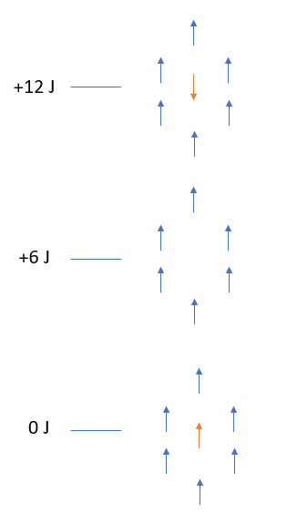
To work this problem out, the schematic in Figure 1 below was drawn and used. Change in energy is New Energy - Old Energy. In the ground state, where all spins are parallel, the system is taken to be in the ground state and is given the conventional value of 0J. Flipping one of the spins can be studied most simply by assuming its a two step process.

First, the central spin is removed altogether thereby removing 6 favourable parallel spin interactions and raising the energy of the system by 6J (again assuming that strength of each interaction is 1J.

Secondly, the antiparallel spin is introduced to the system which adds 6 dis-favourable interactions and therefore further increases the energy of the system by 6J.

The overall energy change is an increase of 12J.

To discuss the gain in entropy we again consider the multiplicity of the system before and after. Multiplicity after spin flip is 1000 as there are 1000 possible sites where the spin flip could occur.

$DeltaS=kln(1000)=9.53X10$^-23

Figure 1: Illustration of the energetic consequences of spin flip in a system.

TASK: Calculate the magnetisation of the 1D and 2D lattices in the figure below. What magnetisation would you expect to observe for an Ising lattice with $$\begin{gathered} D=3, \\ N=1000 \end{gathered}$$ at absolute zero?

Figure 2: Illustration of an Ising lattice in one (N=5), two (N=5x5), and three (N=5x5x5) dimensions. Red cells indicate the "up" spin", and blue cells indicate the "down" spin.

Magnetisation is given by the formula below:

$M=\sum _i{s}_i$

For the 1-D system and the 2-D system, $M=+1$

At absolute 0, the system will be at the lowest possible state which corresponds to either $M=+1000$ or $M=-1000$

Calculating the energy and magnetisation

TASK: complete the functions energy() and magnetisation(), which should return the energy of the lattice and the total magnetisation, respectively. In the energy() function you may assume that $J=1.0$ at all times (in fact, we are working in reduced units in which $J=k_B$, but there will be more information about this in later sections). Do not worry about the efficiency of the code at the moment — we will address the speed in a later part of the experiment.

    def energy(self):
        "Return the total energy of the current lattice configuration."
        J = 1.0
        row = []
        interactions = 0
        energy = 0
        for i in range(0, self.n_rows):
            row = row + [self.lattice[i]*self.lattice[i-1]]
            #essential to use [i-1] rather than [i+1] as python interprets index [i-1] as the last member of the lattice.
            for j in range(0, self.n_cols):
                interactions = interactions + (self.lattice[i][j]*self.lattice[i][j-1])
                #keeps adding on the sideways interactions
        interactions = interactions + np.sum(row)
        energy = -1*J*interactions
        return energy

    def magnetisation(self):
        "Return the total magnetisation of the current lattice configuration."
        magnetisation=np.sum(self.lattice)
        return magnetisation

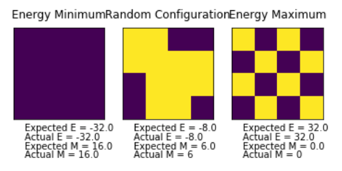
TASK: Run the ILcheck.py script from the IPython Qt console using the command

%run ILcheck.py

The displayed window has a series of control buttons in the bottom left, one of which will allow you to export the figure as a PNG image. Save an image of the ILcheck.py output, and include it in your report.

Figure 3: Testing the functions.

Introduction to the Monte Carlo Simulation

TASK: How many configurations are available to a system with 100 spins? To evaluate these expressions, we have to calculate the energy and magnetisation for each of these configurations, then perform the sum. Let's be very, very, generous, and say that we can analyse $1\times 10^9$ configurations per second with our computer. How long will it take to evaluate a single value of ${⟨M⟩}_T$?

Number of configurations available to a system with 100 spins is 2¹⁰⁰ which is 1.267X10³⁰. This means time by computer to evaluate this would be 1.267X10²¹ seconds which is also 4.366X10¹³ years. This is definitely an unreasonably high computational cost.

TASK: Implement a single cycle of the above algorithm in the montecarlocycle(T) function. This function should return the energy of your lattice and the magnetisation at the end of the cycle. You may assume that the energy returned by your energy() function is in units of $k_B$! Complete the statistics() function. This should return the following quantities whenever it is called: $<E>,<E^2>,<M>,<M^2>$, and the number of Monte Carlo steps that have elapsed.

    def montecarlostep(self, T):
        # complete this function so that it performs a single Monte Carlo step
        energy = self.energy()
        #the following two lines will select the coordinates of the random spin for you
        random_i = np.random.choice(range(0, self.n_rows))
        random_j = np.random.choice(range(0, self.n_cols))
        self.lattice[random_i][random_j] = -self.lattice[random_i][random_j]
        energy_diff = self.energy() - energy
        random_number = np.random.random()
        #this will choose a random number in the range[0,1)
        if random_number > np.exp(-energy_diff/T):
            self.lattice[random_i][random_j] = -self.lattice[random_i][random_j]
        self.E = self.E + self.energy()
        self.M = self.M + self.magnetisation()
        self.E2 = self.E2 + self.energy()**2
        self.M2 = self.M2 + self.magnetisation()**2
        self.n_cycles = self.n_cycles + 1
        return(self.energy(), self.magnetisation())
            
    def statistics(self):
        # complete this function so that it calculates the correct values for the averages of E, E*E (E2), M, M*M (M2), and returns them
        mean_E = self.E/self.n_cycles
        mean_E2 = (self.E2)/self.n_cycles
        mean_M = self.M/self.n_cycles
        mean_M2 = self.M2/self.n_cycles
        return(mean_E , mean_E2 , mean_M , mean_M2)

TASK: If $T<T_C$, do you expect a spontaneous magnetisation (i.e. do you expect $⟨M⟩\ne 0$)? When the state of the simulation appears to stop changing (when you have reached an equilibrium state), use the controls to export the output to PNG and attach this to your report. You should also include the output from your statistics() function.

Figure 4: Result of animation.

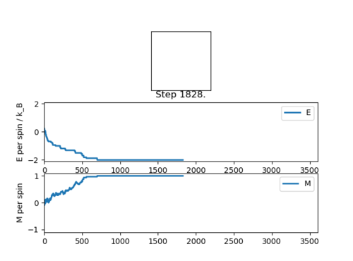
Above the Curie temperature, materials lose their intrinsic magnetic properties which get replaced by induced magentic properties. This promotes haphazard and random electron spin.

At temperatures below the Curie temperature, magnetic moments are aligned and total magnetisation is non-zero and therefore can be said to have spontaneous magnetisation.

Accelerating the code

TASK: Use the script ILtimetrial.py to record how long your current version of IsingLattice.py takes to perform 2000 Monte Carlo steps. This will vary, depending on what else the computer happens to be doing, so perform repeats and report the error in your average!

Average Time Taken from 5 repeats : 9.235286621 s with error 0.1083311793 s

TASK: Look at the documentation for the NumPy sum function. You should be able to modify your magnetisation() function so that it uses this to evaluate M. The energy is a little trickier. Familiarise yourself with the NumPy roll and multiply functions, and use these to replace your energy double loop (you will need to call roll and multiply twice!).

    def energy(self):
        "Return the total energy of the current lattice configuration."
        energy = -(np.sum(np.multiply(self.lattice(np.roll(self.lattice(1,0))))))-
        (np.sum(np.multiply(self.lattice(np.roll(self.lattice(1,1))))))
        return energy

    def magnetisation(self):
        "Return the total magnetisation of the current lattice configuration."
        magnetisation=np.sum(self.lattice)
        return magnetisation

TASK: Use the script ILtimetrial.py to record how long your new version of IsingLattice.py takes to perform 2000 Monte Carlo steps. This will vary, depending on what else the computer happens to be doing, so perform repeats and report the error in your average!

Average Time Taken from 5 repeats: 0.508653721 s with error 0.01732847498 s

Investigating the effect of Temperature

TASK: The script ILfinalframe.py runs for a given number of cycles at a given temperature, then plots a depiction of the final lattice state as well as graphs of the energy and magnetisation as a function of cycle number. This is much quicker than animating every frame! Experiment with different temperature and lattice sizes. How many cycles are typically needed for the system to go from its random starting position to the equilibrium state? Modify your statistics() and montecarlostep() functions so that the first N cycles of the simulation are ignored when calculating the averages. You should state in your report what period you chose to ignore, and include graphs from ILfinalframe.py to illustrate your motivation in choosing this figure.

Several finalframe runs were carried out and it was observed that as the lattice size and temperature were increased, number of steps required to reach equilibrium also increased. Since the smallest lattice size studied (2X2) took 20,000 steps to reach equilibrium, that is number of cycles chosen to be ignored by default so as to save computational cost (time). However, instead of directly generalising how many cycles to ignore, an additional condition was added. Only if the standard deviation in energy was less than 5% from the mean, the new energy and magnetisations were recorded. The code is explained further below using the comments.

    def montecarlostep(self, T):
        energy_list=[]
        self.n_cycles = self.n_cycles + 1
        self.steps=self.steps+1
        energy = self.energy()
        #the following two lines will select the coordinates of the random spin for you
        random_i = np.random.choice(range(0, self.n_rows))
        random_j = np.random.choice(range(0, self.n_cols))
        self.lattice[random_i,random_j] = -self.lattice[random_i,random_j]
        energy_diff = self.energy() - energy
        random_number = np.random.random()
        #this will choose a random number in the range[0,1)
        if energy_diff > 0:
            if random_number > np.exp(-energy_diff/T):
                self.lattice[random_i,random_j] = -self.lattice[random_i,random_j]
        energy_list=energy_list+[energy]    
        
        while (self.steps<20000):
            #This number of steps was minimum number of steps to ignore before reaching equilibrium 
              as seen by testing a 2X2 lattice at T=5
            #As lattice size and temperature were increased, number of steps to equilibrate increased.
            energy = self.energy()
            #the following two lines will select the coordinates of the random spin
            random_i = np.random.choice(range(0, self.n_rows))
            random_j = np.random.choice(range(0, self.n_cols))
            self.lattice[random_i,random_j] = -self.lattice[random_i,random_j]
            energy_diff = self.energy() - energy
            random_number = np.random.random()
            #this will choose a random number in the range[0,1)
            if energy_diff > 0:
                if random_number > np.exp(-energy_diff/T):
                    self.lattice[random_i,random_j] = -self.lattice[random_i,random_j]
            energy_list=energy_list+[energy]
            self.steps=self.steps+1

        i=0
        if self.steps==20000:
            while i==0:
                if np.std(energy_list)>abs(0.05*np.mean(energy_list)):
                    #this condition was added to make the process of ignoring steps more rigorous and automized.
                    #that is, if the standard deviation is more than 5% of the mean, the calculation is run but not made a note of
                    #the following two lines will select the coordinates of the random spin for you
                    random_i = np.random.choice(range(0, self.n_rows))
                    random_j = np.random.choice(range(0, self.n_cols))
                    self.lattice[random_i,random_j] = -self.lattice[random_i,random_j]
                    energy_diff = self.energy() - energy
                    random_number = np.random.random()
                    #this will choose a random number in the range[0,1)
                    if energy_diff > 0:
                        if random_number > np.exp(-energy_diff/T):
                            self.lattice[random_i,random_j] = -self.lattice[random_i,random_j]
                    energy_list=energy_list+[energy]
                    self.steps=self.steps+1
                if np.std(energy_list)<abs(0.05*np.mean(energy_list)):
                    #this  meets the criterion set to start keeping records of energy and 
                    magnetisation in order to correct the averages.
                    i=1
            
        self.E = self.E + self.energy()
        self.M = self.M + self.magnetisation()
        self.E2 = self.E2 + self.energy()**2
        self.M2 = self.M2 + self.magnetisation()**2   
        return(self.energy(), self.magnetisation())
        
    def statistics(self):
        #no modification was required for this as the Monte Carlo Step function only records the energies and magnetisations
        that we are interested in
        mean_E = self.E/self.n_cycles
        mean_E2 = self.E2/self.n_cycles
        mean_M = self.M/self.n_cycles
        mean_M2 = self.M2/self.n_cycles
        no_cycles=self.n_cycles
        return(mean_E, mean_E2, mean_M, mean_M2, no_cycles)

TASK: Use ILtemperaturerange.py to plot the average energy and magnetisation for each temperature, with error bars, for an $8\times 8$ lattice. Use your intuition and results from the script ILfinalframe.py to estimate how many cycles each simulation should be. The temperature range 0.25 to 5.0 is sufficient. Use as many temperature points as you feel necessary to illustrate the trend, but do not use a temperature spacing larger than 0.5. The NumPy function savetxt() stores your array of output data on disk — you will need it later. Save the file as 8x8.dat so that you know which lattice size it came from.

In order to plot the error bars, ILtemperaturerange.py was edited in order to make another running list of standard deviations of energy and magnetisation. These were appended after each monte carlo step and using the generated lists, standard errors were calculated. The code below shows specifically the changes made to the given script and the relevant sections.

Estddev=[]
Mstddev=[]
#added to have a running list of standard deviations

for t in temps:
    Elist=[]
    Mlist=[]
    il = IsingLattice(n_rows, n_cols)
    il.lattice = np.ones((n_rows, n_cols))
    for i in times:
        if i % 100 == 0:
            print(t, i)
        energy, magnetisation = il.montecarlostep(t)
        Elist.append(energy/spins)
        Mlist.append(magnetisation/spins)
    Estddev.append(np.std(Elist))
    Mstddev.append(np.std(Mlist))
    #keep adding to the list created as monte carlo steps are run 
    Merr=np.asarray(Mstddev)/((len(Mlist))**0.5)
    Eerr=np.asarray(Estddev)/((len(Elist))**0.5)
    #calculate standard errors 
fig = pl.figure()

enerax.errorbar(temps, np.array(energies)/spins, yerr=np.asarray(Eerr))
#plot error bars for energies 
magax.plot(temps, np.array(magnetisations)/spins)
magax.errorbar(temps, np.array(magnetisations)/spins,yerr=np.asarray(Merr))
#plot error bars for magnetisations

Each simulation was run for 100,000 cycles with a spacing of 0.01. Although a larger number of cycles would make the obtained averages more accurate, it would take too long on very small lattice sizes let alone a more realistic case where one might want to test larger lattice sizes. This number was chosen keeping computational feasibility in mind.

Also, the strict condition posed in the Monte Carlo step for accepting configurations made it more logical to reduce necessary number of cycles.

Although spacing of 0.25 and 0.1 were tested, it was found that a spacing on 0.01 gave the best illustration of trends.

Investigating effect of system size

TASK: Repeat the final task of the previous section for the following lattice sizes: 2x2, 4x4, 8x8, 16x16, 32x32. Make sure that you name each datafile that your produce after the corresponding lattice size! Write a Python script to make a plot showing the energy per spin versus temperature for each of your lattice sizes. Hint: the NumPy loadtxt function is the reverse of the savetxt function, and can be used to read your previously saved files into the script. Repeat this for the magnetisation. As before, use the plot controls to save your a PNG image of your plot and attach this to the report. How big a lattice do you think is big enough to capture the long range fluctuations?

The representative Jupyter Notebook scripts below show how data was extracted from files and used for plotting Energy and Magnetisation per spin for the different lattice sizes.

datanew=loadtxt("220.01.dat")
temp_2 = datanew[: , 0]
energy_2 = datanew[: , 1]/4
plot(temp_2 , energy_2)
xlabel("Temperature")
ylabel("Energy per spin")
title("Energy per Spin versus Temperature for lattice size 2X2")
savefig('E_OG_22')

datanew=loadtxt("220.01.dat")
temp_2 = datanew[: , 0]
mag_2 = datanew[: , 3]/4
plot(temp_2 , mag_2)
xlabel("Temperature")
ylabel("Magnetisation per spin")
title("Magnetisation per Spin versus Temperature for lattice size 2X2")
savefig('M_OG_22')

Graph 1: Energy per spin for a 2X2 Lattice.

Graph 2: Energy per spin for a 4X4 Lattice.

Graph 3: Energy per spin for a 8X8 Lattice.

Graph 4: Energy per spin for a 16X16 Lattice.

Graph 5: Energy per spin for a 32X32 Lattice.

Graph 6: Magnetisation per spin for a 2X2 Lattice.

Graph 7: Magnetisation per spin for a 4X4 Lattice.

Graph 8: Magnetisation per spin for a 8X8 Lattice.

Graph 9: Magnetisation per spin for a 16X16 Lattice.

Graph 10: Magnetisation per spin for a 32X32 Lattice.

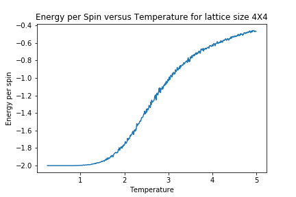
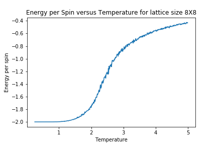
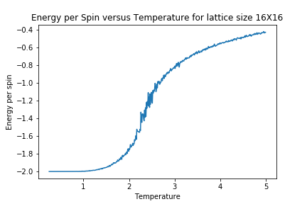
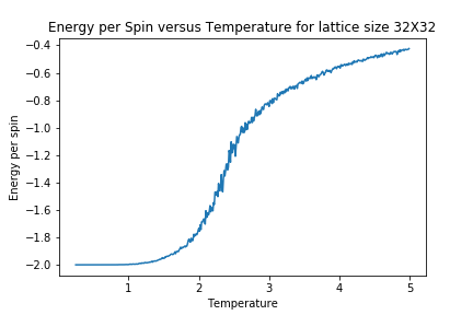
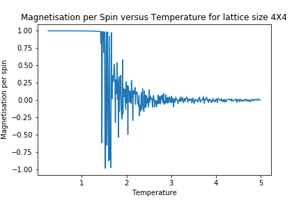
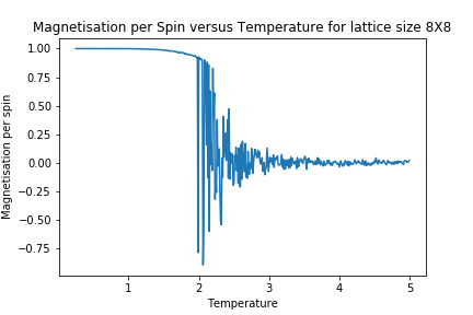
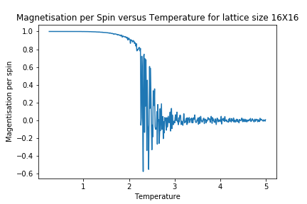
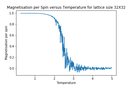
In order to better observe the impact of lattice size upon magnetisation and energy, the following Graphs were generated.

Graph 11: Comparing Energy per spin for different lattice sizes

Graph 12: Comparing Magnetisation per spin for different lattice sizes

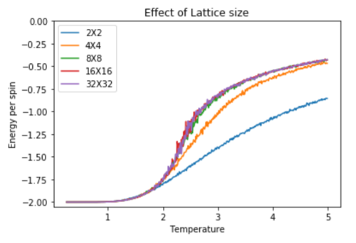
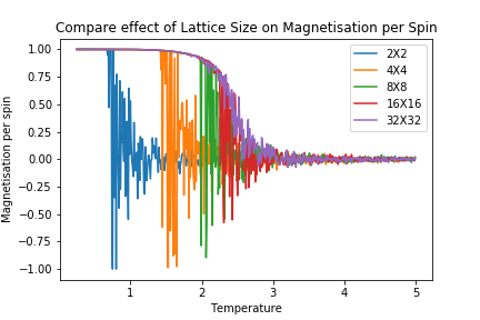
As lattice size is increased, the curvature of the energy plot increases and hints towards a phase transition although not very clearly. The magnetisation comparison is more interesting however. For small lattice sizes such as 2X2, 4X4 and even 8X8, the magnetisation can be seen to be flipping between -1 and 1 well below the curie temperature before dropping to a value of 0. This could be due the small energy barrier for the lattice to adopt either of the ground state spin configurations. On comparison to other Monte Carlo Studies performed on similar lattice sizes, this was not seen in magnetisation plots. The Figure below represents results by Jacques Kotse The observation therefore points towards numerical errors within the study performed.

Figure 5: Plot of Magnetisation versus temperature for different lattice sizes

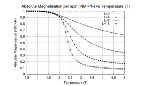
In molecular simulations, long range fluctuations are proportional to the inverse root of N (number of spins) which in our case is the lattice size. Therefore as lattice size increases, we would expect long rage fluctuations to appear and matter less and less. A 32X32 lattice size is big enough to dim down these fluctuations as can be seen above and therefore the biggest lattice size investigated that can capture these fluctuations is a 16X16 lattice.

Determining the Heat Capacity

TASK: By definition,

$C=\frac{\partial ⟨E⟩}{\partial T}$

From this, show that

$C=\frac{\mathrm{V}\mathrm{a}\mathrm{r}[E]}{k_B{T}^2}$

(Where $\mathrm{V}\mathrm{a}\mathrm{r}[E]$ is the variance in $E$.)

Figure 6: Derivation of Heat Capacity in terms of Variance.

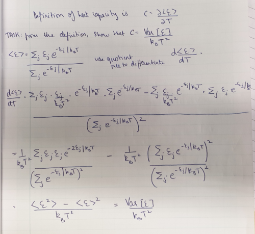
Using this relation, and the data that you generated in the previous sections, you can now determine the heat capacity of your lattice as a function of temperature and system size.

TASK: Write a Python script to make a plot showing the heat capacity versus temperature for each of your lattice sizes from the previous section. You may need to do some research to recall the connection between the variance of a variable, $\mathrm{V}\mathrm{a}\mathrm{r}[X]$, the mean of its square $⟨X^2⟩$, and its squared mean ${⟨X⟩}^2$. You may find that the data around the peak is very noisy — this is normal, and is a result of being in the critical region. As before, use the plot controls to save your a PNG image of your plot and attach this to the report.

def heatc(e,e2,temp,s):
#define a function that determines heat capacity when given inputs of Energy (e),
Energy<sup>2</sup>, Temperature (temp) and Lattice Size (s).
    variance=e2-(e**2)
    heatc=variance/(temp**2)
    return heatc/(s**2)

HC2=heatc(E2,Esq2, temp2,2)

plot(temp2,HC2)
title('Heat capacity per spin vs Temperature: 2x2')
xlabel('Temp')
ylabel('Heat capacity')
savefig('HC_og_22')

Graph 13: Heat capacity for a 2X2 lattice.

Graph 14: Heat capacity for a 4X4 lattice.

Graph 15: Heat capacity for a 8X8 lattice.

Graph 16: Heat capacity for a 16X16 lattice.

Graph 17: Heat capacity for a 32X32 lattice.

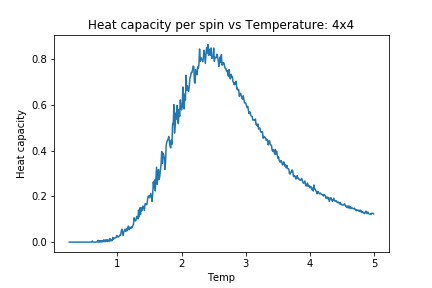
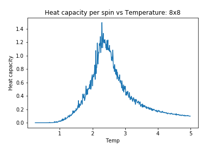
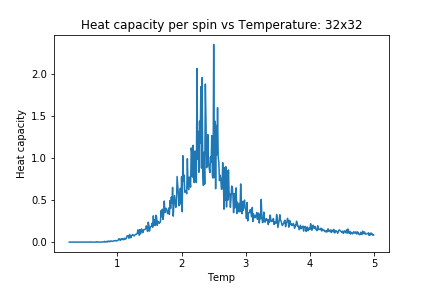
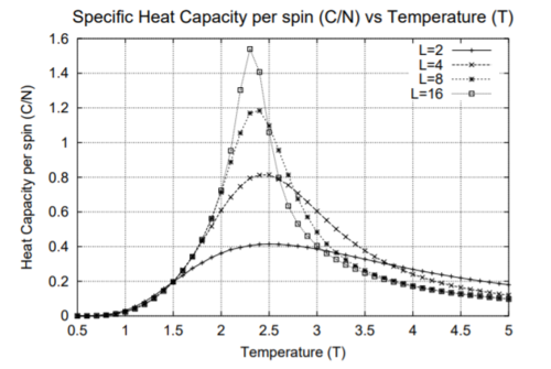
As lattice size is increased, the heat capacity plots become more peaked but at the same time, the region of interest becomes more and more noisy. Upon comparison of this to the aforementioned study there is significant disagreement in the extent of fluctuations and noise. One similarity however, is that both sets of results are far from the expected theoretical divergence at curie temperature.

Figure 7: Heat capacity versus temperature for different lattice sizes.

Locating the Curie Temperature

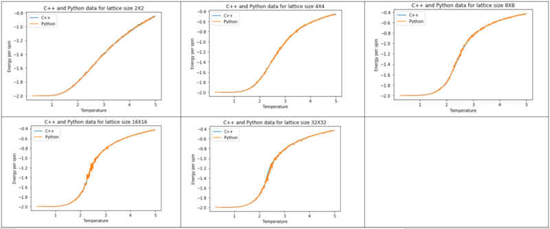
TASK: A C++ program has been used to run some much longer simulations than would be possible on the college computers in Python. You can view its source code here if you are interested. Each file contains six columns: $T,E,E^2,M,M^2,C$ (the final five quantities are per spin), and you can read them with the NumPy loadtxt function as before. For each lattice size, plot the C++ data against your data. For one lattice size, save a PNG of this comparison and add it to your report — add a legend to the graph to label which is which. To do this, you will need to pass the label="..." keyword to the plot function, then call the legend() function of the axis object (documentation here).

The code and figures below show the comparison of C++ and Python data for Energy and Magnetisation

c_2=loadtxt("2X2.dat")
#loading the C++ data provided.
c_temp2 = c_2[:,0]
c_energy2 = c_2[:,1]
plot(c_temp2, c_energy2 , label = "C++")
plot(temp_2 , energy_2 , label = "Python")
xlabel("Temperature")
ylabel("Energy per spin")
title("C++ and Python data for lattice size 2X2")
legend(loc='upper left')
show()
savefig('ak8916_comp_E_22')

Table 1: Comparison of Energy per spin for Python and C++ data.

c_mag2 = c_2[: , 3]
#calling the magentisation data from the C++ files
mag_2 = datanew[: , 3]/4
#calling the magnetisation data from Python data file and 
turning it into per spin by dividing by lattice size squared
plot(temp_2 , mag_2 , label = "Python")
plot(c_temp2, c_mag2 , label = "C++")

xlabel("Temperature")
ylabel("Magnetisation per spin")
title("C++ and Python data for lattice size 2X2")
legend(loc='upper right')
show()
#savefig('ak8916_comp_M_22')

Table 2: Comparison of Magnetisation per spin for Python and C++ data.

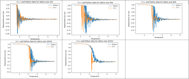
Comparing the C++ and Python generated data

Seeing the comparison graphs for Energy and Magnetisation, it can be observed that as the system size increased, deviation between the produced graphs for these properties also increased. This could be a potential limitation of the way the simulation works in comparison to the C++ program.

Polynomial fitting

TASK: write a script to read the data from a particular file, and plot C vs T, as well as a fitted polynomial. Try changing the degree of the polynomial to improve the fit — in general, it might be difficult to get a good fit! Attach a PNG of an example fit to your report.

As the lattice size was increased, a better fit required very high degree polynomials. Hence, a representative plot of a 2X2 lattice is given below.

data2=loadtxt('HT2n.dat')
#reading the file and extracting relevant columns
T2 = data2[:,0]
H2 = data2[:,1]
#first we fit the polynomial to the data
fit = np.polyfit(T2, H2, 6) # fit a sixth order polynomial

#now we generate interpolated values of the fitted polynomial over the range of our function
T2_min = np.min(T2)
T2_max = np.max(T2)
T_range2 = np.linspace(T2_min, T2_max, 10000) #generate 1000 evenly spaced points between T_min and T_max
fitted_C2_values = np.polyval(fit, T_range2) # use the fit object to generate the corresponding values of C
plot(T2, H2 , label = "Initial Heat Capacity")
plot(T_range2, fitted_C2_values, label = "Fitted Heat Capacity")
legend()
title("Fitting of Heat Capacity for 2X2 lattice")
xlabel("Temperature")
ylabel("Heat Capacity")
show()

Graph 16: Fitting the heat capacity for a 2X2 lattice.

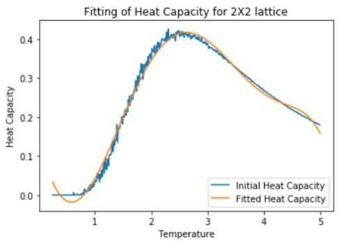
Fitting in a particular temperature range

TASK: Modify your script from the previous section. You should still plot the whole temperature range, but fit the polynomial only to the peak of the heat capacity! You should find it easier to get a good fit when restricted to this region.

A new function fitting_HC() was defined to produce these plots as shown below.

def fitting_HC(T2,H2,T2_min,T2_max,n):
    new_temp=[]
    new_C=[]
    #Temperature max and min were chosen depending on where the peak in heat capacity was found to be.
    T2_min = 2 
    T2_max = 3 
    #The code creates an empty list and divides up the graph into three separate sections to cover the whole temperature range
    #The first section appends the lists of new_temp and new_C with values corresponding to temperatures below the peak region
    i=0
    min_temp_selection = np.logical_and(T2 < T2_min, i==i )
    min_T2_values = T2[min_temp_selection]
    min_H2_values = H2[min_temp_selection]
    new_temp=new_temp+list(min_T2_values)
    new_C=new_C+list(min_H2_values)

    #The second section corresponds to the peak region and uses the previous code to fit the data.
    selection = np.logical_and(T2 > T2_min, T2 < T2_max) #choose only those rows where both conditions are true
    peak_T2_values = T2[selection]
    peak_H2_values = H2[selection]

    fit = np.polyfit(peak_T2_values, peak_H2_values, 3) 

    T_range2 = np.linspace(T2_min, T2_max, 1000) #generate 1000 evenly spaced points between T2_min and T2_max
    fitted_C2_values = np.polyval(fit, T_range2) #use the fit object to generate the corresponding values of C

    new_temp=new_temp+list(T_range2)
    new_C=new_C+list(fitted_C2_values)

    #The third section adds values corresponding to temperatures outside the peak region to list new_temp and new_c
    max_temp_selection = np.logical_and(T2 > T2_max,i==i)
    max_T2_values = T2[max_temp_selection]
    max_H2_values = H2[max_temp_selection]
    new_temp=new_temp+list(max_T2_values)
    new_C=new_C+list(max_H2_values)
    
    plot(new_temp, new_C, label = "Fitted Heat Capacity")
    legend()
    xlabel("Temperature")
    ylabel("Heat Capacity")
    title("Fitting of Heat Capacity for "+str(n)+' lattice')
    return

The plot below shows the result obtained from executing the following function.

fitting_HC(T2,H2,2,3,'2x2')

Graph 17: Partial fitting of heat capacity for a 2X2 lattice.

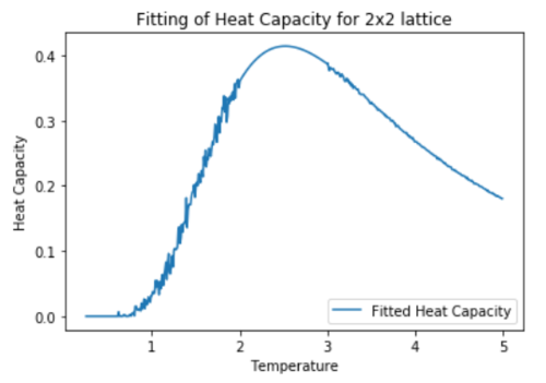
Finding the peak in C

TASK: find the temperature at which the maximum in C occurs for each datafile that you were given. Make a text file containing two colums: the lattice side length (2,4,8, etc.), and the temperature at which C is a maximum. This is your estimate of $T_C$ for that side length. Make a plot that uses the scaling relation given above to determine $T_{C,\mathrm{\infty }}$. By doing a little research online, you should be able to find the theoretical exact Curie temperature for the infinite 2D Ising lattice. How does your value compare to this? Are you surprised by how good/bad the agreement is? Attach a PNG of this final graph to your report, and discuss briefly what you think the major sources of error are in your estimate.

In order to calculate the curie temperature, the following theory was used:

the temperature at which the heat capacity has its maximum must scale according to $T_{C,L}=\frac{A}{L}+T_{C,\mathrm{\infty }}$, where $T_{C,L}$ is the Curie temperature of an $L\times L$lattice, $T_{C,\mathrm{\infty }}$ is the Curie temperature of an infinite lattice, and $A$ is a constant in which we are not especially interested.

Graph 18: Linear Fit plot of Obtained Curie Temperature versus Inverse of Lattice Sizes.

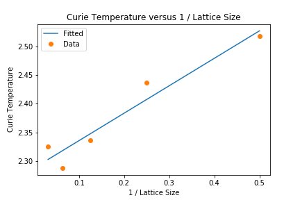
The linear fit for the plot gives the the intercept and hence Curie temperature of 2.29 J/Kb. This compares to the value of 2.26 J/Kb as reported in another Ising model study using the Metropolis Monte Carlo Method. The numerical estimate is quite close to theory and hence proves to be a good alternative to performing exact calculations.

However, the study performed is found to overestimate the curie temperature. This means that the gradient of the generated plot must be steeper to be closer to the theoretical value. This could be a numerical error and possible due to improper scaling of results with increase in system size.

The use of Monte Carlo Simulations to study this method is quite reasonable as the study of Curie Temperature does not require time to be a variable. However, the system does have its limitations.

1. Number of systems studied within the range.

The curie temperature is obtained from the y-intercept of the best fit curve. This automatically implies that a plot with more points (i.e. studying more lattice sizes) would give a better estimate of $T_{C,\mathrm{\infty }}$.

2. Length of simulations (number of Monte Carlo steps) and computational cost to perform them.

Although longer run times and cycles would give a better data for the average, it is computationally too expensive to run the simulations and more number of processors would be required to get better results. The given data generated by C++ came from running much longer simulations and was considerably less noisy than the data generated by Python and therefore confirms this point to be a significant source of error in the calculated value.

3. Finite size of lattice systems studied.

Finite size of lattice limits our ability to clearly pin point the temperature at which the phase transition takes place. Theoretically, this should be the point of divergence in the heat capacity plot. The extent of fluctuations in this region make it unlikely to predict this crucial temperature accurately. The tasks were performed on rather small systems to begin with which represents one of the shortcomings of the model and hence the estimated $T_{C,\mathrm{\infty }}$.

Conclusions

In conclusion, the simulation lab highlighted several not only computational but theoretical concepts regarding ferromagnetism, temperature and statistical thermodynamics.

The difficulty in achieving an exact solution for the Curie temperature of an infinite lattice using a Monte Carlo Simulation derived from the direct relationship between accuracy of the simulation with system size and number of Monte Carlo steps. However, the approach worked well to illustrate interesting physical trends and behaviour of the spin system.

Looking further on, it would be interesting to explore some of the other applications of the Monte Carlo Method to study slow systems such as diffusion of long chain polymers.

References

- ↑ Mańka, A., Nowicki, W. & Nowicka, G. J Mol Model (2013) 19: 3659. https://doi.org/10.1007/s00894-013-1875-z
- ↑ Laosiritaworn, W.; Laosiritaworn, Y. Time Resolved Effect of Heat Dispersion on Magnetic Stability in Ferromagnetic Ising Thin-Films: Monte Carlo Simulation. Journal of Magnetics 2012, 17 (4), 233–241 DOI: 10.4283/jmag.2012.17.4.233.
- ↑ Ayache, L.; Tahiri, N.; Ez-Zahraouy, H. Monte Carlo study of a layering transition with spin-1 Blume–Capel model under crystal field effect. Physica A: Statistical Mechanics and its Applications 2019, 513, 734–741 DOI: 10.1016/j.physa.2018.08.131.
- ↑ Kadiri, A., Ngantso, G.D., EL Amraoui, Y. et al. J Supercond Nov Magn (2018) 31: 4047. https://doi.org/10.1007/s10948-018-4677-9
- ↑ Kotze, Jacques. (2008). Introduction to Monte Carlo methods for an Ising Model of a Ferromagnet.
- ↑ file:///C:/Users/ak8916/Downloads/Khudier.pdf Curie Temperature is reported as 2.27 KbT.
- ↑ http://web.mit.edu/krish_s/www/files/ising_Model.pdf