Rep:Aab1817 Monte Carlo

Introduction to the Ising model

1. Show that the lowest possible energy for the Ising model is $$\begin{gathered} E \\ = \\ -DNJ \end{gathered}$$, where D is the number of dimensions and N is the total number of spins. What is the multiplicity of this state? Calculate its entropy.

We know that the energy is given by $$\begin{gathered} -\frac{1}{2}J\sum _i^N\sum _{j \\ \in \\ \mathrm{n}\mathrm{e}\mathrm{i}\mathrm{g}\mathrm{h}\mathrm{b}\mathrm{o}\mathrm{u}\mathrm{r}\mathrm{s}\left(i\right)}{s}_i{s}_j \end{gathered}$$. For the lowest energy state, we have a system with all spins either up or down. If we start with a model where D=1 and N=4, we get 8 possible interactions. Because all the spins are the same, this illustrates how the sum term of the energy is equal to 8, and we can relate it to 2DN, it this case 2 x 1 x 4. Since we have figured out that $$\begin{gathered} \sum _i^N\sum _{j \\ \in \\ \mathrm{n}\mathrm{e}\mathrm{i}\mathrm{g}\mathrm{h}\mathrm{b}\mathrm{o}\mathrm{u}\mathrm{r}\mathrm{s}\left(i\right)}{s}_i{s}_j \end{gathered}$$ equals 2DN, $$\begin{gathered} \frac{1}{2}\sum _i^N\sum _{j \\ \in \\ \mathrm{n}\mathrm{e}\mathrm{i}\mathrm{g}\mathrm{h}\mathrm{b}\mathrm{o}\mathrm{u}\mathrm{r}\mathrm{s}\left(i\right)}{s}_i{s}_j \end{gathered}$$ must equal DN. Hence, we obtain the expression mentioned above, where the lowest possible energy is given by E= - DNJ.

The multiplicity of the state refers to the number of possible combination it can adopt: as mentioned before, the system could have all of its spins up or all of its spins down. The multiplicity is thus 2. The entropy is linked to the multiplicity by the relation $S=k_B\ln \mathrm{\Omega }$, we get $S=k_b\ln (2)$

2. Imagine that the system is in the lowest energy configuration. To move to a different state, one of the spins must spontaneously change direction ("flip"). What is the change in energy if this happens (D=3,\ N=1000)? How much entropy does the system gain by doing so?

Adopting a similar reasoning pattern to that of the previous question, if all spins were the same, the sum term of the energy would be equal to 2DN, so 6000. But by flipping one of the spins, we will have 12 terms in the summation that will change from +1 to -1, that is 6 terms for the interactions of the flipped spin with its neighbours, and 6 for the interactions of the neighbours with the flipped spin. Now we have 5988 terms in the sum equaling +1 and 12 terms equaling -1. The sum term is now equal to 5976, and from that we get the value of the energy of the new system: $E=-\frac{1}{2}J\times 5976=-2988J$.

The lowest energy is $E_0=-3000J$

The energy change is thus $\mathrm{\Delta }E=12J$

The entropy of the system is $S=k_B\ln (2000)$, because there are 1000 spins to choose from when wanting to change one, and we could start with either all spins being up or down. The entropy gain is thus $\mathrm{\Delta }S=k_B\ln (1000)$

3. Calculate the magnetisation of the 1D and 2D lattices in figure 1. What magnetisation would you expect to observe for an Ising lattice with D = 3,\ N=1000 at absolute zero?

Figure 1: Illustration of an Ising lattice in one (N=5), two (N=5x5), and three (N=5x5x5) dimensions. Red cells indicate the "up" spin", and blue cells indicate the "down" spin. Taken from the script's wiki.

Based on the image provided in the script we have:

for the 1D case, $M=\sum _i{s}_i=1+1+1-1-1=+1$

for the 2D case, $M=\sum _i{s}_i=13-12=+1$

For the case in which D=3, N=1000, and T=0K. At this temperature, we assume the system takes the lowest energy configuration. $M=\sum _i{s}_i=1000$ or $M=\sum _i{s}_i=-1000$

Calculating the energy and magnetisation

1. complete the functions energy() and magnetisation(), which should return the energy of the lattice and the total magnetisation, respectively. In the energy() function you may assume that J=1.0 at all times (in fact, we are working in reduced units in which J=k_B, but there will be more information about this in later sections). Do not worry about the efficiency of the code at the moment — we will address the speed in a later part of the experiment.

The functions were completed as follows:

   def energy(self):
       "Return the total energy of the current lattice configuration."
       energy=0.0
       for i in range(0,self.n_rows):
           for j in range(0, self.n_cols):
               if i == self.n_rows-1 and j == self.n_cols-1:
                   energy += self.lattice[self.n_rows-1,self.n_cols-1]*self.lattice[1,self.n_cols-1]
                   energy += self.lattice[self.n_rows-1, self.n_cols-1]*self.lattice[self.n_rows-1,1]
              elif j == self.n_cols-1:
                  energy += self.lattice[i,self.n_cols-1]*self.lattice[i+1,self.n_cols-1]
                  energy += self.lattice[i,self.n_cols-1]*self.lattice[i,1]
              elif i == self.n_rows-1:
                  energy+= self.lattice[self.n_rows-1,j]*self.lattice[self.n_rows-1,j+1]
                  energy += self.lattice[self.n_rows-1,j]*self.lattice[1,j]
              else:
                  energy+= self.lattice[i,1]*self.lattice[i+1,j]
                  energy += self.lattice[i,j]*self.lattice[i,j+1]
       energy*= 1.0 # multiply by constant J=1.0
       return energy

    def magnetisation(self):
         "Return the total magnetisation of the current lattice configuration."
         magnetisation=0.0
         for i in self.lattice:
             for j in i:
                 magnetisation += np.float(j)
         return magnetisation

2.Run the ILcheck.py script from the IPython Qt console using the command %run ILcheck.py The displayed window has a series of control buttons in the bottom left, one of which will allow you to export the figure as a PNG image. Save an image of the ILcheck.py output, and include it in your report.

Figure 2': Output figure of the ILcheck.py file, which confirms the validity of the code above.

Introduction to Monte Carlo simulation

1. How many configurations are available to a system with 100 spins?

For a system of $n$ distinguishable particles that can attain one of two possible spin states, there are $2^n$ different spin configurations. Hence for 100 particles, there are $2^{100}$ possible configurations, which evaluated is approximately 1.2676506e+30.

To evaluate these expressions, we have to calculate the energy and magnetisation for each of these configurations, then perform the sum. Let's be very, very, generous, and say that we can analyse 1\times 10^9 configurations per second with our computer. How long will it take to evaluate a single value of ${⟨M⟩}_T?$

The time needed to calculate a single value of ${⟨M⟩}_T$ is the possible number of configurations divided by the computation speed. This evaluate to roughly <10^{21}</math> seconds.

2. Implement a single cycle of the above algorithm in the montecarlocycle(T) function. This function should return the energy of your lattice and the magnetisation at the end of the cycle. You may assume that the energy returned by your energy() function is in units of k_B! Complete the statistics() function. This should return the following quantities whenever it is called: <E>, <E^2>, <M>, <M^2>, and the number of Monte Carlo steps that have elapsed.

The function was defined as follows:

   def montecarlostep(self,T):
       energy =self.energy()
       random_i= np.random.choice(range(0, self.n_rows))
       random_j= np.random.choice(range(0,self.n_cols))
       self.lattice[random_i, random_j] *= -1
       energy1= self.energy()
       E_diff=energy1-energy
       if E_diff<0:
             energy =energy1
      else:
           R=np.random.random()
           if R <= np.exp(-E_diff/T):
               energy=energy1
           else:
                energy=energy
      self.energies.append(energy)
      self.__magnetisations.append(self.magnetisation())
      self.n_cycles +=1
      return energy, self.magnetisation()

Where self.energies, self.__magnetisations, and self.n_cycles are defined at the top of the class, outside the Monte Carlo function.

The statistics function was defined as follows:

   def statistics(self):
       energies= np.asarray(self.energies)
       magnetisations= np.asarray(self.__magnetisations)
       E=np.mean(energies)
       E2= np.mean(np.power(energies,2))
       M= np.mean(magnetisations)
       M2= np.mean(magnetisations**2)
       return E, E2, M, M2, self.n_cycles

3. If $T<T_C$, do you expect a spontaneous magnetisation (i.e. do you expect $⟨M⟩\ne 0$)? When the state of the simulation appears to stop changing (when you have reached an equilibrium state), use the controls to export the output to PNG and attach this to your report. You should also include the output from your statistics() function.

For a temperature under the Curie temperature, the spins are more likely to adapt a random configuration, i.e. random distribution of -1 and +1, which results in a value of M close to zero. Above the Curie temperature, the system loses its permanent properties, so under a magnetic field, the spins are likely to point in the same direction, leading to higher values of M.

By animating our simulation, we see that the value of M tends to approach zero at low temperatures.

Figure 3': Output figure of the ILanim.py file, plotting energy and magnetisation per spin against number of steps taken

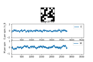
Averaged quantities: E = 0.0421478060046 E*E = 0.26457852194 M = 0.018920804465 M*M = 0.0170845812885

Averaged quantities: E = 0.0125921890714 E*E = 0.0311936913342 M = 0.0126340931948 M*M = 0.0176704450218

Accelerating the code

1. Use the script ILtimetrial.py to record how long your current version of IsingLattice.py takes to perform 2000 Monte Carlo steps. This will vary, depending on what else the computer happens to be doing, so perform repeats and report the error in your average!

Before improving the code, it takes $2.76687630769\pm 0.052078053156$ seconds to perform 2000 Monte Carlo steps.

2. Look at the documentation for the NumPy sum function. You should be able to modify your magnetisation() function so that it uses this to evaluate M. The energy is a little trickier. Familiarise yourself with the NumPy roll and multiply functions, and use these to replace your energy double loop (you will need to call roll and multiply twice!).

The functions were modified as follows:

   def energy(self):
        energy=0.0
        rows= len(self.lattice)
        columns= len(self.lattice[0])
        for m in range(rows):
            for n in range(columns):
                energy += np.multiply(self.lattice[0][0],self.lattice[0][1])
                energy += np.multiply(self.lattice[0][0], self.lattice[1][0])
                self.lattice= np.roll(self.lattice,1,axis=1)
            self.lattice= np.roll(self.lattice,1,axis=0)
        return energy

    def magnetisation(self):
       magnetisation=0.0
       for i in self.lattice:
            magnetisation += np.sum(i)
       return magnetisation

3. Use the script ILtimetrial.py to record how long your new version of IsingLattice.py takes to perform 2000 Monte Carlo steps. This will vary, depending on what else the computer happens to be doing, so perform repeats and report the error in your average!

After the code improvement, the computation time is of $2.7336015\pm 0.0145477689686$ seconds.

The effect of temperature

1. The script ILfinalframe.py runs for a given number of cycles at a given temperature, then plots a depiction of the final lattice state as well as graphs of the energy and magnetisation as a function of cycle number. This is much quicker than animating every frame! Experiment with different temperature and lattice sizes. How many cycles are typically needed for the system to go from its random starting position to the equilibrium state? Modify your statistics() and montecarlostep() functions so that the first N cycles of the simulation are ignored when calculating the averages. You should state in your report what period you chose to ignore, and include graphs from ILfinalframe.py to illustrate your motivation in choosing this figure.

The number of cycles needed to reach the equilibrium state is taken as N=1500. This was chosen as the number of steps required for the average values of energy and magnetisation to reach their expected convergence, i.e. for magnetisation, zero.

The functions were modified in the following way:

  def montecarlostep(self,T):
      energy =self.energy()
      random_i= np.random.choice(range(0, self.n_rows))
      random_j= np.random.choice(range(0,self.n_cols))
      self.lattice[random_i, random_j] *= -1
      energy1= self.energy()
      E_diff=energy1-energy
      if E_diff<0:
            energy =energy1
     else:
          R=np.random.random()
          if R <= np.exp(-E_diff/T):
              energy=energy1
          else:
               energy=energy
     if self.n_cycles <= 1500:
         self.energies= self.energies
     else:
         self.energies.append(energy)
         self.__magnetisations.append(self.magnetisation())
         self.n_cycles +=1
     return energy, self.magnetisation()

    def statistics(self):
           energies= np.asarray(self.energies)
           magnetisations= np.asarray(self.__magnetisations)
           E=np.mean(energies)
           E2= np.mean(np.power(energies,2))
           M= np.mean(magnetisations)
           M2=np.mean(magnetisations**2)
       return  E, E2, M, M2, (self.n_cycles-1500)

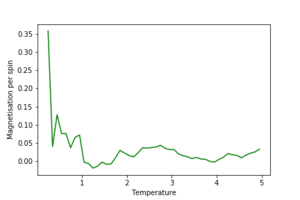
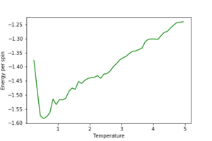
2. Use ILtemperaturerange.py to plot the average energy and magnetisation for each temperature, with error bars, for an 8\times 8 lattice. Use your intuition and results from the script ILfinalframe.py to estimate how many cycles each simulation should be. The temperature range 0.25 to 5.0 is sufficient. Use as many temperature points as you feel necessary to illustrate the trend, but do not use a temperature spacing larger than 0.5. The NumPy function savetxt() stores your array of output data on disk — you will need it later. Save the file as 8x8.dat so that you know which lattice size it came from.

Figure 5': Average magnetisation per spin against temperature for an 8x8 lattice

Figure 4': Average energy per spin against temperature for an 8x8 lattice

The effect of system size

1. Repeat the final task of the previous section for the following lattice sizes: 2x2, 4x4, 8x8, 16x16, 32x32. Make sure that you name each datafile that your produce after the corresponding lattice size! Write a Python script to make a plot showing the energy per spin versus temperature for each of your lattice sizes. Hint: the NumPy loadtxt function is the reverse of the savetxt function, and can be used to read your previously saved files into the script. Repeat this for the magnetisation. As before, use the plot controls to save your a PNG image of your plot and attach this to the report. How big a lattice do you think is big enough to capture the long range fluctuations?

Figure 6': Average energy per spin against temperature for different lattice sizes

Figure 7': Average magnetisation per spin against temperature for different lattice sizes

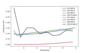
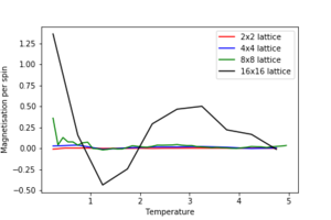
The estimated minimum lattice size is at least 16x16, potentially larger, as we see major improvement in accounting for larger fluctuations.

Determining the heat capacity

1. By definition, $C=\frac{\partial ⟨E⟩}{\partial T}$. From this, show that $C=\frac{\mathrm{V}\mathrm{a}\mathrm{r}[E]}{k_B{T}^2}$ (Where $\mathrm{V}\mathrm{a}\mathrm{r}[E]$ is the variance in E.)

$<E>=\sum _j{p}_j{ϵ}_j$ where$p_j=\frac{e^{-}{ϵ}_j\beta }{Z}$ and $Z$ is the partition function.

$<E>=-\frac{1}{Z}\frac{dZ}{d\beta }=-\frac{d\ln (Z)}{d\beta }=U$ $(\mathrm{\Delta }E{)}^2=<E^2>-<E{>}^2$ but $<E^2>=\frac{d^{2}Z}{d{\beta }^2}$

$(\mathrm{\Delta }E{)}^2=\frac{d^2\ln (Z)}{d{\beta }^2}=-\frac{dU}{d\beta }=-\frac{dU}{dT}\frac{dT}{d\beta }=k_B{T}^2\frac{dU}{dT}=k_B{T}^{2}C$

Thus, $(\mathrm{\Delta }E{)}^2=Var[E]=k_b{T}^{2}C$

2. Write a Python script to make a plot showing the heat capacity versus temperature for each of your lattice sizes from the previous section. You may need to do some research to recall the connection between the variance of a variable, $\mathrm{V}\mathrm{a}\mathrm{r}[X]$, the mean of its square $⟨X^2⟩$, and its squared mean ${⟨X⟩}^2$. You may find that the data around the peak is very noisy — this is normal, and is a result of being in the critical region. As before, use the plot controls to save your a PNG image of your plot and attach this to the report.

Figure 8': Heat capacity against temperature for different lattice sizes

Locating the Curie temperature

1. A C++ program has been used to run some much longer simulations than would be possible on the college computers in Python. You can view its source code here if you are interested. Each file contains six columns: T, E, E^2, M, M^2, C (the final five quantities are per spin), and you can read them with the NumPy loadtxt function as before. For each lattice size, plot the C++ data against your data. For one lattice size, save a PNG of this comparison and add it to your report — add a legend to the graph to label which is which.

Figure 9': Comparison of the experimental vs the given C++ data for a 8x8 lattice

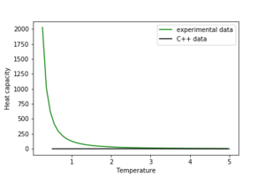
The discrepancy in the plot shows that the experimental data needs correction, but both exhibit a peak in heat capacity.

2.Write a script to read the data from a particular file, and plot C vs T, as well as a fitted polynomial. Try changing the degree of the polynomial to improve the fit — in general, it might be difficult to get a good fit! Attach a PNG of an example fit to your report.

With the C++ data already imported, it was fitted as such:

   T = eightc[:,0] #get the first column
   C = eightc[:,5] # get the second column
   #first we fit the polynomial to the data
   fit = np.polyfit(T, C, 3) # fit a third order polynomial
   #now we generate interpolated values of the fitted polynomial over the range of our function
   T_min = np.min(T)
   T_max = np.max(T)
   T_range = np.linspace(T_min, T_max, 1000) #generate 1000 evenly spaced points between T_min and T_max
   fitted_C_values = np.polyval(fit, T_range) # use the fit object to generate the corresponding values of C
   plt.plot(eightc[:,0],eightc[:,5],'k', label="C++ data")
   plt.plot(T_range,fitted_C_values,'b', label="fit")
   plt.xlabel("Temperature")
   plt.ylabel("Heat capacity")
   plt.legend()
   plt.show()

Figure 10': Fitted polynomial for the whole range of temperature of the C++ data for a 8x8 lattice

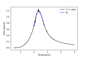
3. Modify your script from the previous section. You should still plot the whole temperature range, but fit the polynomial only to the peak of the heat capacity! You should find it easier to get a good fit when restricted to this region.

The region for which the data was fitted was T=[2.0,2.8]°K

It was fitted as follows:

   T = eightc[:,0] #get the first column
   C = eightc[:,5] # get the second column
   Tmin = 2.0 
   Tmax = 2.8 
   #now we generate interpolated values of the fitted polynomial over the range of our function
   selection = np.logical_and(T > Tmin, T < Tmax) #choose only those rows where both conditions are true
   peak_T_values = T[selection]
   peak_C_values = C[selection]
   #first we fit the polynomial to the data
   fit = np.polyfit(peak_T_values, peak_C_values, 3) # fit a third order polynomial
   fitted_C_values = np.polyval(fit, peak_T_values) # use the fit object to generate the corresponding values of C
   plt.plot(eightc[:,0],eightc[:,5],'k', label="C++ data")
   plt.plot(peak_T_values,fitted_C_values,'b', label="fit")
   plt.xlabel("Temperature")
   plt.ylabel("Heat capacity") 
   plt.legend()
   plt.show()

Figure 10': Fitted polynomial for the whole range of temperature of the C++ data for a 8x8 lattice

4. Find the temperature at which the maximum in C occurs for each datafile that you were given. Make a text file containing two colums: the lattice side length (2,4,8, etc.), and the temperature at which C is a maximum. This is your estimate of $T_C$ for that side length. Make a plot that uses the scaling relation given above to determine $T_{C,\mathrm{\infty }}$. By doing a little research online, you should be able to find the theoretical exact Curie temperature for the infinite 2D Ising lattice. How does your value compare to this? Are you surprised by how good/bad the agreement is? Attach a PNG of this final graph to your report, and discuss briefly what you think the major sources of error are in your estimate.

Figure 11': Fitted polynomial for the whole range of temperature of the C++ data for a 8x8 lattice

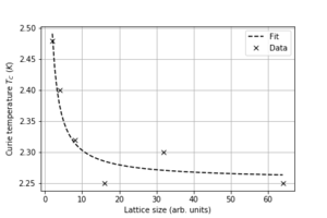
Using the following code:

   twomax= np.max(twoc[:,5])
   Tmax2 = twoc[:,0][twoc[:,5] == twomax]
   fourmax= np.max(fourc[:,5])
   Tmax4 = fourc[:,0][fourc[:,5] == fourmax]
   eightmax= np.max(eightc[:,5])
   Tmax8 = twoc[:,0][eightc[:,5] == eightmax]
   sixtmax= np.max(sixtc[:,5])
   Tmax16 = sixtc[:,0][sixtc[:,5] == sixtmax]
   thirtmax= np.max(thirtc[:,5])
   Tmax32 = thirtc[:,0][thirtc[:,5] == thirtmax]
   sixtymax= np.max(sixtyc[:,5])
   Tmax64 = sixtyc[:,0][sixtyc[:,5] == sixtymax]
   c= np.array([twomax,fourmax, eightmax,sixtmax, thirtmax, sixtymax])
   L = np.array([2,4,8,16,32,64])
   t=np.array([Tmax2, Tmax4, Tmax8, Tmax16, Tmax32, Tmax64]).flatten()
   from scipy.optimize import curve_fit
   def func(x, a, b):
       return a/x + b
   popt, pcov = curve_fit(func, L, t)
   l = np.linspace(L[0],L[-1],100)
   plt.plot(l, func(l, *popt), 'k--', label='Fit')
   plt.plot(L, t, "kx", label="Data")
   plt.grid()
   plt.legend()
   plt.xlabel("Lattice size (arb. units)")
   plt.ylabel(r"Curie temperature $T_C$ ($K$)")
   plt.show()

We get that the experimental Curie temperature is $2.25616915\pm 0.01593072$ Kelvin.

The Kramers-Wannier duality gives one possible relationship for the Curie temperature.

$T_c/J=\frac{2}{\ln (1+\sqrt{2})}\approx 2.26918531421.$

Hence, the value extracted from the data is similar, within error to the theoretical value.