Transition Structures and Reactivity

Experiment Overview

In this experiment, Gaussian 5.0, a popular software used for computational chemistry, was used to study the Cope rearrangement of 1,5-hexadiene and also the Diels-Alder cycloadditions of ethylene with butadiene and maleic anhydride with cyclohexa-1,3-diene.

For the Cope rearrangement, the main aims were to (a) determine the lowest energy conformation of 1,5-hexadiene and (b) locate the transition state structure(s) for the rearrangement. For the Diels-Alder cycloadditions, this research aimed to (a) determine the transition state structures and (b) study the molecular orbitals that interact in the transition state. Specific to the maleic anhydride + cyclohexa-1,3-diene system, an explanation to the stereoselectivity of the product (exo- vs. endo-adduct) was sought.

A list of the .log files for the calculations run in this experiment can be found here.

A Brief Introduction to the Calculations

When running a calculation, the Gaussian program must solve the electronic Schrodinger equation $(\hat{h} ψ_{i} = e_{i} ψ_{i})$ ^[1]. To do this, it is required that the method (i.e. the level of theory used to solve the electronic Schrodinger equation) and type of calculation be specified.

Three different methods were used in this experiment and are referred to throughout this report; HF/3-21G, B3LYP/6-31G* and AM1. The simplifications applied by the Hartree-Fock method (HF) include the Born-Oppenheimer approximation and the simplification of the complex many-electron wavefunction of the system to a Slater determinant of one-electron wavefunctions ^[2]. Density Functional Theory (DFT) adds a level of complexity to the HF method by including an exchange-correlation potential term to the electronic energy calculation. HF neglects this term and so DFT calculations provide a more accurate result for the energy of a system at the cost of longer calculation times. This term (or 'functional') can be defined, with the most popular choice being B3LYP (Becke, 3-parameter, Lee-Yang-Parr) ^[3]. The last method is AM1 (Austin Model 1) ^[4]. This is a semi-empirical method based on HF which approximates certain integrals that are calculated in HF to zero and estimates the important ones based on experimental data ^[1]. This has the result of significantly reducing calculation times.

Nf710 (talk) 13:54, 24 February 2016 (UTC) A slater determinant is not 1 electron, its is antisymetrised amny electron determinant which makes all the electrons in the system indistingusable.

The 3-21G and 6-31G* refer to the type of basis sets used in the calculation. This input is required for most methods, but not semi-empirical methods like AM1 ^[5]. There are many different types of basis sets which can be used - read more here.

The two key types of calculations run in this experiment were opt and freq, with a third (IRC) introduced later. The first refers to the geometry optimisation of an input structure to a critical point on the potential energy surface. Depending on what is specified in Gaussian, a opt calculation can be used to find low energy conformations of a molecule (minima on the PES) or a transition state structure (maxima). The freq keyword computes the force constants, vibrational frequencies and associated infrared intensities. This is done after a geometry optimisation and is useful in determining what type of critical point has been located.

Nf710 (talk) 13:54, 24 February 2016 (UTC) A good brief understanding of the methods. you could have gone into more detail though.

The Cope Rearrangement

In this section we will focus on the Cope rearrangement of 1,5-hexadiene (Figure 1). The Cope rearrangement is a very well-known example of a [3,3]-sigmatropic rearrangement, a type of pericyclic reaction in which there appears to be a movement of a sigma bond from one position of a molecule to another position in the same molecule (Δσ = 0). Historically, there has been some debate as to the mechanism of this rearrangement, with evidence supporting either a concerted mechanism with an 'aromatic'-like transition state or a stepwise/'asynchronous' radical mechanism proceeding via a biradical intermediate ^[6]. It is now generally accepted that the rearrangement occurs via a concerted mechanism with a 6-membered 'chair' or 'boat' transition state. This section outlines the computational study of various conformations of the diene and the two possible transition states.

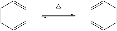Figure 1: The Cope rearrangement of 1,5-hexadiene
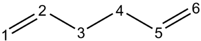Figure 2: Numbering scheme for 1,5-hexadiene used in this report

Conformations of 1,5-hexadiene

Initially, a molecule of 1,5-hexadiene with an antiperiplanar (app) conformation with respect to the central C-C sigma bond (C3-C4) was drawn. The Modify Dihedral tool in GaussView was used to ensure an absolute angle of 180 ° (i.e. exactly app). The molecule was cleaned with the Clean function and subsequently optimised at the HF/3-21G level. The resulting structure and its energy are shown in Table 1 below. Using the Symmetrize tool, the point group of the molecule was found to be C₂.

Table 1

Conformation

Structure

Energy (HF/3-21G)

Anti structure, orientated along the C3-C4 bond to highlight the app arrangement of the double bonds

Energy = -145389.33408 kcal mol^-1

Following the methods outlined to generate the anti structure above, a molecule of 1,5-hexadiene in a gauche conformation was optimised at the HF/3-21G level. The dihedral angle was set to an absolute angle of 60 °. Again, a C₂ point group was determined. The following table displays the results obtained.

Table 2

Conformation

Structure

Energy (HF/3-21G)

Gauche structure, orientated along the C3-C4 bond to highlight the gauche arrangement of the double bonds

Energy = -145388.74699 kcal mol^-1

From comparison of the energies and point groups of the two structures optimised above with the table for conformers provided, it can be seen that the Anti 1 and the Gauche 2 structures have been found. The energies are identical to 5 decimal places which is sufficient since the decimal places beyond this are not significant. Since a more negative value of total energy corresponds to a more stable structure, Anti 1 is the lower energy conformer of the two structures optimised above. Based on the what is known from the conformational analysis of n-butane ^[7], the gauche structure would be expected to be less stable than the anti. This is due to steric strain arising from having the two double bonds (the two 'largest' groups) being too close in space when the dihedral angle = 60 °.

The Lowest Energy Conformation

From the table for conformers, it can be seen that Gauche 3 is the most stable conformer. This was initially a surprising result since, based on the steric strain argument, it was assumed that, in general, anti conformers should be lower in energy than gauche conformers. This assumption likely originated from only considering rotation around the C3-C4 bond, however rotation around the C2-C3 and C4-C5 bonds are also possible. Consequently, the rotational minima of all three bonds must be considered and the problem is not as simple as it initially seemed.

As a first approximation, with considering the possibility of rotation about the C2-C3 and C4-C5 bonds, it was thought the anti conformer in which the double bonds are co-planar could be the lowest energy conformer. The results of the calculations are displayed in Table 3. They show this conformer, which has C_2h symmetry, is in fact one of the highest in energy. The structure drawn is not included in the table for conformers, however it is most similar to Anti 3 in this table and conformer 'K' in literature ^[8] ^[9]. The results are consistent with literature in showing this anti conformer is not the global minimum at any level of theory, suggesting that arguments based only on sterics are insufficient and further considerations are required.

Table 3

Conformation

Structure

Energy (HF/3-21G)

Co-planar anti structure, orientated along the C3-C4 bond to highlight the app arrangement of the double bonds

Energy = -145384.81215 kcal mol^-1

The Gauche 3 structure was optimised at the HF/3-21G level and the point group confirmed to be C₁. The results are shown in Table 4.

Table 4

Conformation

Structure

Energy (HF/3-21G)

Energy (B3LYP/6-31G*)

Gauche 3 structure, orientated along the C3-C4 bond to highlight the gauche arrangement of the double bonds

Energy = -145389.37102 kcal mol^-1

Energy = -147220.86125 kcal mol^-1

The reason that the Gauche 3 conformer is the lowest in energy has been attributed to CH/π interaction ^[8]. This is a stereoelectronic interaction of the π bonding orbital of one C=C bond (HOMO) with the σ* vinyl C-H bond (LUMO) of the other double bond ^[10]. Clearly, this effect sufficiently stabilises the system such that the molecule can overcome the unfavourable sterics of the gauche interactions and preferentially adopts this conformation. Figure 3 illustrates the CH/π interaction possible in this gauche conformer.

The molecule was then re-optimised at the B3LYP/6-31G* level (energy results shown in Table 4) and the molecular orbitals (MOs) calculated. Looking through the MOs for this conformer, an MO that exactly resembles this interaction could not be found. However, the MO corresponding to the highest occupied molecular orbital (HOMO) of the molecule showed some bonding interaction between the π orbitals of two double bonds (Figure 4). The geometry of the Gauche 3 conformer brings the two double bonds closer together allowing this stabilising through-space interaction which could not be easily obtained, for example, in the co-planar anti structure shown previously in this section.

Nf710 (talk) 14:01, 24 February 2016 (UTC) This drawing is fantastic! also excellent arguement for bond rotation at room temperature! This clearly explain the energy lowering with the use of MOs well done!

Figure 3: Illustration of the CH/π interaction for the Gauche 3 conformer of 1,5-hexadiene
Figure 4: The HOMO (MO 23) for the Gauche 3 conformer

A comparison of the geometry of the calculated Gauche 3 structures with literature ^[11] can be found in Table 5. These literature values were obtained experimentally through electron diffraction studies of gaseous 1,5-hexadiene at room temperature. For the values obtained from computation, the standard errors are provided in brackets where appropriate. At both the HF/3-21G and B3LYP/6-31G* levels of theory, all the parameters quite closely agree to experiment as they are usually within experimental error (the values in brackets for the Literature Value column). For some parameters, the HF/3-21G structure is closer to experiment, namely the C(H2)-C(H2)-C(H) angles, whereas for other parameters the B3LYP/6-31G* structure is a better match, especially the C(H)-C(H2)-C(H2)-C(H) dihedral angle.

A particularly important parameter for deducing the conformation of 1,5-hexadiene is the C(H2)=C(H)-C(H2)-C(H2) dihedral angle since it relates the geometry of the double bond relative to the central C-C bond and can therefore be used to eliminate certain conformers (e.g. Anti 3). Unfortunately, since many conformers have values for this dihedral angle of approximately 120 °, the literature data provided is insufficient to conclude whether Gauche 3 is the experimentally preferred conformer for gaseous 1,5-hexadiene. In reality, at room temperature, there is likely sufficient thermal energy (0.5925 kcal mol^-1 at 298.15 K) to overcome the kinetic activation barrier for bond rotation and allow interconversion between conformers. It is highly unlikely the molecule would spend all its time adopting one conformer, especially since many conformers are within 1 kcal mol ^-1 of Gauche 3. The literature data may therefore be considered to apply to an average structure of thermally accessible 1,5-hexadiene conformers.

Table 5
Parameter	Value from HF/3-21G Calculation	Value from B3LYP/6-31G* Calculation	Literature Value ^[11]
Mean C-H Bond Length / Å	1.0791 (± 0.0017)	1.0929 (± 0.0017)	1.087 (± 0.002)
Mean C=C Bond Length / Å	1.3164	1.3337	1.340 (± 0.003)
Mean C(H₂)-C(H) Bond Length / Å	1.5089	1.5046	1.508 (± 0.012)
C(H₂)-C(H₂) Bond Length / Å	1.5532	1.5501	1.538 (± 0.027)
C(H₂)-C(H₂)-C(H) Angle / °	111.7774, 111.8711	109.5086, 113.4622	111.5 (± 0.9)
C(H₂)-C(H)=C(H₂) Angle / °	124.5321, 125.026	124.9341, 125.4946	124.6 (± 1.0)
C(H)-C(H₂)-C(H₂)-C(H) Dihedral Angle / °	67.7022	66.3325	66.3 (Gauche)
C(H₂)=C(H)-C(H₂)-C(H₂) Dihedral Angle / °	120.8625, 117.2146	122.4639, 119.7482	119.7

Nf710 (talk) 14:02, 24 February 2016 (UTC) Excellent compariosn with literature. This is very interesting!

Anti 2 Conformation

Energy and Geometry

The Anti 2 conformer of 1,5-hexadiene was optimised at the HF/3-21G level and confirmed to have a C_i point group. The point group of the molecule was then constrained to C_i using the Point Group Symmetry function before run a DFT reoptimisation at the B3LYP/6-31G* level. The symmetry was maintained in the output of the calculation. The results from both calculations are shown in Table 6. When comparing like-for-like in terms of the calculation method, the energies obtained indicate this conformer is only marginally less stable than the Gauche 3 conformer at both levels of theory.

Table 6

Conformation

Structure

Energy (HF/3-21G)

Energy (B3LYP/6-31G*)

Anti 2 conformation, orientated along the C3-C4 bond to highlight the app arrangement of the double bonds

Energy = -145389.29193 kcal mol^-1

Energy = -147221.10257 kcal mol^-1

Visually, the structures produced from both calculations seem identical, however, when probing the structures using the Modify Bond and Modify Dihedral tools, some differences are noticeable. The results are shown in Table 7. With the higher level of theory (B3LYP/6-31G*), the single bond lengths (e.g. C3-C4) have shortened, relative to the value computed from the HF/3-21G calculation, while the double bonds (C1-C2 & C5-C6) have lengthened. It is unclear why a different calculation method affects the different bonds in different ways. Ultimately, the bond lengths are within error of each other (e.g. approx. 1 % for the C1-C2 bonds) and so there is no significant difference between the two methods. Table 7 shows that the C2-C3-C4-C5 dihedral angle remains at 180 ° across both calculations, as defined prior to running the calculations, meaning the app geometry has been maintained. For a given calculation method, there is no significant difference between the C1-C2-C3-C4 and C3-C4-C5-C6 dihedral angles. The dihedral angles are larger for the B3LYP/6-31G* calculation by approximately 4 °, which is about a 3 % difference relative to the HF/3-21G calculation.

Table 7
	C1-C2 & C5-C6 Bond lengths / Å	C2-C3 & C4-C5 Bond lengths / Å	C3-C4 Bond length / Å	C1-C2-C3-C4 Dihedral Angle / °	C2-C3-C4-C5 Dihedral Angle / °	C3-C4-C5-C6 Dihedral Angle / °
HF/3-21G	1.31617	1.50882	1.55317	114.62785	180.00000	114.62759
B3LYP/6-31G*	1.33350	1.50420	1.54816	118.59948	180.00000	118.59948

Frequency Analysis

Using the optimised B3LYP/6-31G* Anti 2 structure, a frequency calculation was run at the same level of theory. Figure 5 shows the list of calculated normal modes of vibration for this conformer of 1,5-hexadiene and this is translated to the predicted IR spectrum in Figure 6. There are 42 possible vibrations, as predicted from the 3N - 6 rule, where N is the number of atoms (in this case 16). Not all vibrational frequencies appear in the IR spectrum because not all vibrations are IR active. For a vibration to be IR active, there must be a change in the electric dipole moment of the molecule upon absorption of IR radiation. This is a quantum mechanical selection rule for IR spectroscopy ^[12]. Figures 7 and 8 illustrate two vibrations with the greatest intensities in the IR spectrum.

Figure 5: List of the normal modes of vibration for the Anti 2 conformer
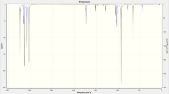Figure 6: IR spectrum simulated for the Anti 2 conformer
Figure 7: The asymmetric C-H stretch found at 3136 cm^-1 (expand to view the animation)
Figure 8: CH₂ wagging found at 940 cm^-1 (expand to view the animation)

From the .log file outputted by the frequency calculation, some thermodynamic quantities can be extracted which, by default, are calculated at 298.15 K and 1 atm (i.e. standard conditions). The key ones are tabulated below (Table 8). The first quantity is the Sum of Electronic and Zero-Point Energies which is the sum of the potential energy of the molecule at 0 K with the zero-point vibrational energy (E₀ = E_elec + ZPE).

Side note on the zero-point energy:

According to quantum mechanics, the zero-point energy is the lowest possible energy a physical system may have. This means that even at 0 K, molecules retain some vibrational energy. This residual energy is a consequence of Heisenberg's Uncertainty Principle

(Δ x Δ ρ (x) \geq \frac{h}{4 π})

which does not allow a particle to remain stationary, even at 0 K, otherwise we would know both the position (

(x)

and momentum

(ρ (x))

of that particle with great precision.

The next quantity is the Sum of Electronic and Thermal Energies. At temperatures above absolute zero, the internal energy of a molecule (U) also has contributions from translational, rotational and vibrational degrees of freedom (U = E₀ + E_trans + E_rot + E_vib). The sum is therefore the energy at a given temperature and pressure (in this case 298.15 K, 1 atm) taking into account these extra contributions. These contributions are calculated from partition functions derived from statistical thermodynamics ^[13].

The Sum of Electronic and Thermal Enthalpies is related to the previous quantity in that the thermal enthalpy, H, is given by H = U + RT (where R is the gas constant). The temperature dependence of this equation means that at temperatures above 0 K, the RT correction term becomes non-negligible. Since RT is always positive, the Sum of Electronic and Thermal Enthalpies should always be more positive than the Sum of Electronic and Thermal Energies, as illustrated in Table 8.

The last quantity, Sum of Electronic and Thermal Free Energies, is calculated using G = H - TS (where G = Gibbs free energy, S = entropy). At 0 K, G = H, however above this temperature, there is an entropic contribution to the free energy which, again, can be calculated from partition functions ^[13].The magnitude of this contribution to the free energy depends on the temperature. Since the absolute entropy of a substance is always positive (or zero for a perfect crystalline solid at absolute zero), TS is always a positive quantity and so the Sum of Electronic and Thermal Free Energies should be more negative than the Sum of Electronic and Thermal Enthalpies. Table 8 illustrates this.

Table 8
	Energy / Hartrees	Energy / kcal mol^-1
Sum of Electronic and Zero-Point Energies	-234.469219	-147131.687710
Sum of Electronic and Thermal Energies	-234.461869	-147127.075514
Sum of Electronic and Thermal Enthalpies	-234.460925	-147126.483145
Sum of Electronic and Thermal Free Energies	-234.500809	-147151.510738

Optimising the Chair and Boat Transition Structures

Chair Optimisation to a TS(Berny)

The chair transition state structure for the Cope rearrangement of 1,5-hexadiene was first estimated using the Berny Optimisation Algorithm. A step-by-step run through of the actions taken during a TS(Berny) optimisation can be found here. This method involves computing the force constant matrix (a Hessian matrix).

The Hessian Matrix:

The Hessian is a second derivative matrix of the system. The first derivative of the energy of the system $(\frac{\partial E (r)}{\partial r})$ gives the gradient of the potential energy surface (PES) with respect to the atomic position, $r$ . Setting this derivative to zero allows critical points (i.e. minima and maxima on the surface) to be located. To determine the nature of a critical point, the second derivative, which corresponds to the curvature of the PES, must be calculated $(\frac{\partial^{2} E (r)}{\partial r_{i} \partial r_{j}})$ . A transition state structure is located at a saddle point on the PES and so a maxima must be located to find this structure. Due to the curvature of a function at its maxima, the second derivative has a negative value. In contrast, a local minima, which for example could correspond to a stable intermediate or product, would have a positive value for the second derivative.

For an accessible but relatively detailed description of the Hessian click here.

For the TS(Berny) optimisation to work correctly, a reasonable guess structure for the transition state must be used as an input. If the initial structure is very different to the structure that makes chemical sense, an 'incorrect' local maxima may be located.

As an reasonable guess for the Cope rearrangement chair transition state, two allyl fragments were used. To start, a CH₂CHCH₂ structure was drawn and optimised at the HF/3-21G level and found to have a C_2v point group (see Table 9).

Table 9

Conformation

Structure

Energy (HF/3-21G)

Allyl (CH₂CHCH₂) fragment used for the proceeding calculation

Energy = -72680.070494 kcal mol^-1

This allyl fragment was copied and pasted twice in a new structure window with one fragment above the other and orientated such that the terminal carbons of the two fragments, but not the central carbons, were in-line. The interatomic distance between the terminal carbons was set (but not fixed) to 2.2 Å. An Opt+Freq calculation, optimised to a TS(Berny), with the force constant calculated Once was run and the result shown in Table 10. The keyword opt=noeigen was added to the calculation to prevent the calculation from potentially crashing if more than one imaginary frequency is calculated.

From Table 10 the deviation of the allyl fragment geometry from planar to a structure with the central carbon slightly raised above (or lowered below) the plane of the terminal carbons is apparent. The individual fragments no longer have a plane of symmetry (σ_v). The chair transition state itself has a C_2h point group.

Table 10

Conformation

Structure

Energy (HF/3-21G)

The chair transition state calculated via optimisation of 2 allyl fragments to a TS (Berny)

Energy = -145343.35018 kcal mol^-1

Figure 9 gives an alternative view of the transition state. This figure displays the similarly between this transition state and the chair conformer of a cyclohexane ring ^[14] when looking at the double Newman projection. It can be seen that all groups are in staggered (gauche) conformations with respect to each other hence reducing torsional strain. Figure 10 gives a partial list of the vibrations calculated for the transition state structure. Unlike in previous calculations, where the molecule was optimised to a minimum, the transition state has a vibration with a negative frequency at -818 cm^-1. This is referred to as the imaginary frequency.

The Imaginary Frequency:

As mentioned previously, the Hessian matrix is calculated in this optimisation and for transition states, the second derivative of the PES is negative. The second derivative of the PES is related to the force constant, $k$ .

$k \propto \frac{\partial^{2} E (r)}{\partial r_{i} \partial r_{j}}$

If a bond can be represented by a quantum harmonic oscillator, the following expression for the vibrational frequency can be used (where $ν$ is the frequency of the oscillator/bond, $k$ is the force constant of the bond and $μ$ is the reduced mass):

$ν = \frac{1}{2 π} \sqrt{\frac{k}{μ}}$

For a negative second derivative, $k$ is negative (let $k = - x$ ). Since $\sqrt{- x} = i \sqrt{x}$ and the reduced mass is always positive, the resulting frequency has a imaginary unit ( $i$ ) hence why the negative frequency found is referred to as the 'imaginary frequency'.

Figure 11 is the animation of this imaginary vibration. The vibration involves the asymmetric C-C stretches of the two sets of terminal carbons. At one extreme of the vibration, i.e. when one C-C bond is shortened (compression) and the other is stretched, the structure resembles the 1,5-hexadiene structure. At the other extreme, the structure also resembles 1,5-hexadiene, however with the central C-C bond in a different place. One extreme can be considered the 'reactant' of the Cope rearrangement and the other extreme the 'product', confirming the 'correct' transition state structure has been located.

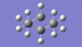Figure 9: View of the transition state to illustrate the chair-like double-staggered 'conformation'
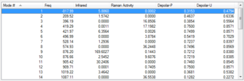Figure 10: List of the normal modes of vibration for the chair TS with the imaginary vibration highlighted
Figure 11: The imaginary vibration found at -818 cm^-1 (expand to view the animation)

Chair Optimisation by the Frozen Coordinate Method

The second method used to locate the Cope rearrangement chair transition state, the Frozen Coordinate Method, also utilised two allyl fragments as the starting point. This time, the atomic distance between the terminal carbons was set and fixed to 2.2 Å using the Redundant Coord Editor. In the .gjf file (input file for a computation), the following lines of code relevant to this method can be found:

B 14 6 2.200000

B 14 6 F

B 9 1 2.200000

B 9 1 F

The letter B refers to a bond meaning the changes being applied affect a specified bond. The following two numbers specific which two atoms to be focused on - in this case, they refer to the terminal carbons. The first and third line of the code have a third number '2.200000'. This is the desired bond length. Therefore, lines 1 and 3 set the bond length between atoms 14 & 6 and 9 & 1 to 2.2 Å. The F in lines 2 and 4 mean Freeze Coordinate and so lines 2 and 4 of the code fix the bond length and coordinates of the atoms specified.

The resulting 'frozen coordinate' structure was optimised to a minimum at the HF/3-21G level. The additional keyword Opt=ModRedundant was automatically inputted to the calculation set-up. The results of the calculation are shown in Table 11. It can be seen that a structure similar to that outputted for the TS(Berny) optimisation previously is produced, however the distance between the terminal carbons has remained at 2.2 Å and consequently the energy is slightly higher.

Table 11
Conformation	Energy (HF/3-21G)
The chair transition state after a frozen coordinate optimisation (to a minimum)	Energy = -145340.75422 kcal mol¹

The output file was again edited with the Redundant Coord Editor to unfreeze the bonds and prepare the structure for the subsequent optimisation to TS(Berny). The following code is found in the .gjf file (where the D refers to Derivative which 'tells' the calculations to use a numerical Hessian):

B 14 6 D

B 9 1 D

In the optimisation, the keyword opt=noeigen was again implemented and the option to calculate the force constants changed to Never. The results are shown in Table 12. The structure, its energy and its imaginary frequency (-817.89cm^-1) are identical to that computed from the TS(Berny) method meaning the correct transition state structure for the Cope rearrangement was located. The bond lengths that were previously fixed have been labelled in the JSmol to show they have decreased to 2.02 Å.

Table 12

Structure

Energy (HF/3-21G)

Energy = -145343.35017 kcal mol^-1

Comparison of Chair TS Geometries

The chair transitions for the Cope rearrangement has been found via two methods; computation of the Hessian (TS(Berny) method) and the Frozen Coordinate method. The geometries of the structures at the HF/3-21G level are compared in Table 13 below. The carbon numbering has been defined according to the structure in Table 12.

Table 13
	C1-C9 Distance / Å	C6-C14 Distance / Å	C1-C4 Bond Length / Å	C4-C6 Bond Length / Å	C1-C4-C6 Angle / °	C9-C12-C14 Angle / °	C4-C1-C9 Angle / °	C4-C6-C14 Angle / °
TS(Berny)	2.0201	2.0199	1.3892	1.3894	120.5008	120.5073	101.8710	101.8652
Frozen Coordinate	2.0207	2.0207	1.3893	1.3893	120.5288	120.5287	101.8469	101.8448

Nf710 (talk) 17:05, 24 February 2016 (UTC) very Nice geometry conversion

The results show that there is no significant difference, at least at this level of theory, between the geometries of the two chair transition states. The C1-C9 and C6-C14 distances are within 0.01 Å across the two methods and are both 2.02 Å (to 3 significant figures).

Since the calculated structures are virtually identical, a comparison of the computational cost for the two methods is appropriate. From Table 10, it can be seen the job cpu time is 8 seconds for the TS(Berny) method. This is contrast to the total job cpu time of 35 seconds for the Frozen Coordinate method (tables 11 and 12). The additional requirement to freeze the geometries and optimise to a minimum for the latter method has quadrupled the computational cost. Assuming that the input guess of a transition state geometry is close enough that only one and not multiple runs of a TS(Berny) optimisation is required, this method may be preferentially chosen over the Frozen Coordinate method.

From these geometries, the nature of bonding can be derived. The C1-C9 and C6-C14 distances are much longer than an average C-C single bond length (1.54 Å, based on diamond ^[15]). In both gauche conformers optimised previously, the distance between the terminal carbons (which ultimately for the single bond after the Cope rearrangement) is calculated to be greater than 4 Å. Using this as a basis, it can be approximated that the distance between the two C=C bonds in 1,5-hexadiene must at least half and the central C-C single bond must significantly elongate for the chair transition state to be reached.

From Table 13, it can also be seen that all other C-C bond lengths are 1.39 Å (to 3 s.f.). This is clearly shorter than an average C-C single bond, but is in fact longer than an average C=C double bond (~ 1.34 Å). This suggests some degree of delocalisation, which is unsurprising since the calculation started with two allyl fragments. Interestingly, this bond length is identical to that for benzene ^[16] and likely explains why the rearrangement is described to occur via an "aromatic-like transition state", as previously stated. Clearly, the transition state structure is not truly aromatic since one of the bond is far too long (2.02 Å) and the structure is not planar.

Boat Optimisation to a TS(QST2)

An alternative method to TS(Berny) was used locate the boat transition state structure for the Cope rearrangement of 1,5-hexadiene - the QST2 method. Rather than working from two allyl fragments, positioned to have all atoms eclipsed, the reactant and product structures are used as inputs. This method interpolates between the two structures to find a transition state structure. (A related method, QST3, also requires a guess transition state structure to be inputted, which may improve the accuracy – read more here.)

Initial Geometries

As an initial approximation, the Anti 2 structure, previously optimised at the HF/3-21G level, was used as the reactant and product. It was necessary to renumber the atoms in both structures so change in connectivity can be tracked by Gaussian (e.g. C3-C4 breaks and C1-C6 forms). An optimisation to TS(QST2) was run at the HF/3-21G level and the results collected in Table 14. Clearly, the calculated transition state structure does not correspond to desired boat transition state. In fact, the energy and the staggered conformation correspond to the chair transition state previously calculated. Furthermore, this structure has bonds between opposite ends of what would be two allyl fragments and therefore makes no chemical sense.

Table 14

Initial Structures

Calculated TS Structure

Energy (HF/3-21G)

Initial reactant and product structures

Energy = -145343.35017 kcal mol^-1

The interpolation has located the incorrect maxima on the PES and this is because the reactant and product structures are too dissimilar to the desired transition state. Clearly, the molecules must be altered such that calculation begins closer to the saddle point on the PES corresponding to the boat transition state.

Altered Geometries

The geometry of the Anti 2 structures were altered so they were closer to the boat transition state structure. The central dihedral angles (i.e. C2-C3-C4-C5 in the reactant and C2-C1-C6-C5 in the product) was changed to 0 ° resulting in an eclipsed conformation. The C2-C3-C4 and C3-C4-C5 angles for the reactant and the corresponding angles in the product molecule were changed to 100 °. The resulting structures can be seen in Initial Structures column of Table 15.

The optimisation to TS(QST2) was re-run and the structure obtained shown in Table 15. The point group of the structure is C_2v. The calculation has clearly converged to the correct structure since there are now 'bonds' between the termini of what would be the two allyl fragments in a way that makes chemical sense. The job cpu time is equal to the TS(Berny) method used for the chair transition state. Hence, it has been shown that, in this case, assuming reasonable input structures are provided, the TS(QST2) method is also preferential to the Frozen Coordinate method in terms of computational cost.

Table 15

Initial Structures

Calculated TS Structure

Energy (HF/3-21G)

Initial reactant and product structures after altering geometries

Energy = -145332.98303 kcal mol^-1

Furthermore, from Figure 12, it can be see how to computed structure closely resembles the boat conformer of cyclohexane (which itself is technically also a transition state in the ring flipping ^[14]). Akin to the lower stability of a cyclohexane boat relative to the cyclohexane chair, the boat transition state of the Cope rearrangement is less stable than the chair transition state. In addition to the torsional strain arising from the unfavourable eclipsed conformation, the boat structure of cyclohexane also suffers steric 'flagpole' interactions which destabilise the structure ^[17].

Figure 13 is the partial list of vibrational modes computed for the transition state structure and it shows a single imaginary frequency. Figure 14 depicts this vibration and, just like in Figure 11, this is the one that corresponds to the Cope rearrangement.

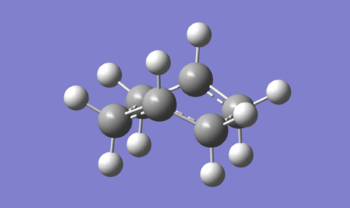Figure 12: View of the transition state to illustrate the boat-like eclipsed 'conformation'
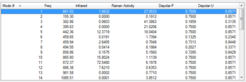Figure 13: List of the normal modes of vibration for the boat TS with the imaginary vibration highlighted
Figure 14: The imaginary vibration found at -841 cm^-1 (expand to view the animation)

Nf710 (talk) 17:06, 24 February 2016 (UTC) Correct frequencies and energeis

Intrinsic Reaction Coordinate

From Figure 9, it may be deduced that the chair transition state most closely resembles the Gauche 2 conformer of 1,5-hexadiene. Similarly, from Figure 12, it could perhaps be postulated that the boat transition state structure could resembles the Anti 2 conformer if the C2-C3-C4-C5 dihedral angle was set to 0 ° to obtain an eclipsed geometry. Though these conformers resemble the transition states, they are not guaranteed to be the conformation that the product molecule (after the Cope rearrangement) will reach. The method used to calculate the local minimum structure from a transition state starting point is called the Intrinsic Reaction Coordinate method. At the transition state structure, we are at local maximum on the PES, as depicted by the crude diagram in Figure 15. Much like a ball rolling down a hill, the IRC calculation takes the structure from the maximum down the PES (the 'hill') to a local minimum via the minimum energy pathway. The 'forward' direction of the IRC is defined as "direction the transition vector is pointing when the largest component of the transition vector (“phase”) is positive" (Reference) – basically, the steepest way down the PES at the saddle point. Since the Cope rearrangement of 1,5-hexadiene is a reversible reaction with the reactant and product molecules being identical, the reaction coordinate is symmetrical and so the forward and 'backward' directions of the IRC are identical.

Figure 15: Diagram to depict the reaction coordinate

Chair Transition State IRC

An IRC calculation in the forward direction for 50 steps was run on the chair transition state structure at the HF/3-21G level. The forward constant was calculated at every step along the IRC. The calculation terminated early (after 44 steps) since the RMS gradient (root mean square) converged to zero – or more technically, the acceptable cut-off value – and so a minimum on the PES was found. The following lines can be found in the log file to confirm this:

PES minimum detected on this side of the pathway.

Magnitude of the gradient = 0.0001433

Calculation of FORWARD path complete.

Figure 16 shows the two curves relevant to IRC calculations. The first is the Total Energy along IRC which shows that as the calculation proceeds, the energy of the structure is decreasing. This is as expected since the calculation starts with a transition state, a high energy species and ends with a more stable intermediate/product structure. The second curve is the RMS gradient Norm along IRC which measures the gradient as the calculation proceeds. At zero reaction coordinate (the start), the gradient is zero since the calculation starts with a transition state structure which exists on a maxima on the PES. The gradient sharply rises as the calculation takes the structure off the saddle point and down the PES slope where it is steepest. The calculation ends with the gradient at zero again since the stable structure found exists in a 'valley' (local minima) on the PES.

Figure 17 illustrates the change in structure from the chair TS to the local minimum 1,5-hexadiene structure and the JSmol to the right shows the final structure obtained from the IRC calculation. From this it can be seen that the Gauche 2 has been located, however the energy was not quite identical to that obtained from earlier calculations (see Figure 18). The structure obtained was optimised at the HF/3-21G to a minimum and the result shown in Figure 19. This energy matches that obtained earlier and confirms the Gauche 2 structure was obtained from the IRC calculation. Upon closer inspection, it was realised that this is actually an enantiomer of Gauche 2 ^[8]

Figure 16: IRC curves outputted for the chair TS to a gauche conformer of 1,5-hexadiene
Figure 17: Animation showing the progression of the IRC calculation (expand to view)
Figure 18: Energy summary for the final structure in the chair IRC
Figure 19: Energy summary after HF/3-21G optimisation to minimum (chair to Gauche 2)

Local minimum energy conformation from the IRC calculation of the chair TS

Boat Transition State IRC

An identical IRC calculation (50 steps) was carried out on the boat transition state structure, however this proved to be an insufficient number of steps since the energy did not converge to zero (see the .log file). The calculation was re-run at 100 steps which was sufficient since the gradient converged to zero in 74 steps. Figure 20 shows the relevant curves for the IRC calculation and Figure 21 is an animation of the IRC. In contrast to Figure 16, which exhibited a smooth decay in the RMS gradient curve to zero, Figure 20 shows a shallow rise in the gradient prior to convergence. This can be attributed to the unique landscape of the PES and likely shows a very small saddle point (or 'bump' on the PES) has been traversed before reaching the local minimum.

The final structure obtained is shown in the JSmol on the right and is evidently the Gauche 3 conformer. This structure was optimised at the HF/3-21G level to a minimum and the energy shown in Figure 23 is seen to be identical to that obtained in early calculations for the Gauche 3 conformer.

Figure 20: IRC curves outputted for the boat TS to a gauche conformer of 1,5-hexadiene
Figure 21: Animation showing the progression of the IRC calculation for the boat TS (expand to view)
Figure 22: Energy summary for the final structure in the boat IRC
Figure 23: Energy summary after HF/3-21G optimisation to minimum (boat to Gauche 3)

Local minimum energy conformation from the IRC calculation of the boat TS

Nf710 (talk) 17:10, 24 February 2016 (UTC) Correct conformer identified

Comparison of Transition States

The chair transition state obtained from the TS(Berny) method and the boat transition state were optimised at the B3LYP/6-31G* level to a TS(Berny). The C-C distances between the terminal carbons of the two allyl fragments have been displayed in Table a. For the chair transition state, the distance has decreased slightly going from HF/3-21G to B3LYP/6-31G*, whereas the inverse trend is seen for the boat transition state. Ultimately, this change is very minor (only about 0.05 Å) and it can be concluded there is no significant change in the geometry of either transition state when re-optimising at the higher level.

Table 16
	Distance (HF/3-21G) / Å	Distance (B3LYP/6-31G*) / Å
Chair TS	2.0199, 2.0201	1.96669, 1.96670
Boat TS	2.13825, 2.13843	2.20639, 2.20640

Activation Energies

Table 17 is a collection of various thermodynamic parameters for the Anti 2 conformer and the two transition states at both levels of theory. Firstly, it can be noted that for all the parameters shown in Table 17, the B3YLP/6-31G* method has produced a more negative energy value than the corresponding value from the HF/3-21G method. Relative to the reactant, both the chair and boat transition states are higher in energy and this is as expected since it agrees with the chemical intuition that a transition state is a unisolable high energy, unstable species which is formed on the way to the products.

Table 17
	HF/3-21G			B3YLP/6-31G*
	Electronic Energy / Hartrees	Sum of Electronic and Zero-Point Energies (0 K) / Hartrees	Sum of Electronic and Thermal Energies (298.15 K) / Hartrees	Electronic Energy / Hartrees	Sum of Electronic and Zero-Point Energies (0 K) / Hartrees	Sum of Electronic and Thermal Energies (298.15 K) / Hartrees
Anti 2 Conformer (Reactant)	-231.69253517	-231.539539	-231.532566	-234.61171062	-234.469219	-234.461869
Chair TS	-231.61932235	-231.466697	-231.461338	-234.55693104	-234.414908	-234.408980
Boat TS	-231.60280125	-231.450919	-231.445293	-234.54307883	-234.402356	-234.396012

The following table gives the activation energies for the chair and boat transition states at two temperatures, computed at the two levels of theory. The Activation Energy at 0 K has been calculated by subtracting the Sum of Electronic and Zero-Point Energies (0 K) (in Table 17) of the reactant from the Sum of Electronic and Zero-Point Energies (0 K) of the appropriate transition state. Equally, the Activation Energy at 298.15 K has been calculated from the appropriate Sum[s] of Electronic and Thermal Energies (298.15 K). These values show how much higher the transition state are in energy relative to Anti 2. It is evident that the boat transition state is always higher in energy than the chair (approx. 10 kcal mol^-1 at HF/3-21G and 8 kcal mol^-1 at B3LYP/6-31G*). The factors that destabilise the boat have been discussed previously. This result confirms that for the Cope rearrangement, it is energetically more favourable to proceed via the chair transition state than the boat since the energy barrier is smaller.

It can also be seen that the Activation Energy at 298.15 K is always approximately 1 kcal mol^-1 lower than the corresponding Activation Energy at 0 K (e.g. 33.19 kcal mol^-1 vs. 34.08 kcal mol^-1 for ΔE_chair at B3LYP/6-31G*). Perhaps this indicates that the energy barrier to get from Anti 2 to the transition state is lowered by translational, rotational and vibrational contributions when thermal energy is provided to the system.

Table 18
	HF/3-21G		B3LYP/6-31G*
	Activation Energy at 0 K / kcal mol^-1	Activation Energy at 298.15 K / kcal mol^-1	Activation Energy at 0 K / kcal mol^-1	Activation Energy at 298.15 K / kcal mol^-1
ΔE^‡_chair	45.71	44.70	34.08	33.19
ΔE^‡_boat	55.61	54.76	41.96	41.33

Comparison to literature values for the activation energy is useful in determining the accuracy of these computed values. The literature values, based on experiment are ΔH^‡_chair = 33.5 (± 0.5) kcal mol^-1 and ΔH^‡_boat = 44.7 (± 2.0) kcal mol^-1 ^[18]. The uncertainty values are standard deviations. Recalling that H = U + RT, ΔH^‡ = ΔU^‡ since at constant temperature, the correctional terms (RT) cancel out. This allows direct comparison with values in Table 18. Clearly, the results of the B3LYP/6-31G* calculations more closely agree with experiment – particularly for the the chair transition state where the Activation Energy at 298.15 K is within error of literature and the Activation Energy at 0 K is almost within error. The agreement is less close for the boat transition state where, for example, the Activation Energy at 298.15 K is 3 % off the lower bound of the literature value.

As discussed in the introduction, the B3YLP/6-31G* method gives a more accurate result for the electronic energy than HF/3-21G and this has been demonstrated in tables 17 and 18. The previous section also illustrated how the geometries are virtually identical at both levels of theory. This leads to the conclusion that optimisation at the HF/3-21G is sufficient if the geometry/conformation of a system is of interest and so unnecessary computational costs of re-optimisation can be avoided. However, to obtain more accurate thermodynamic properties, optimisation at the B3LYP/6-31G* level is required.

Nf710 (talk) 17:15, 24 February 2016 (UTC) very good good report. Lovely figures and everything is very well explained. You could have gone into more detail on the theorey of the computational methods however everything else was excellent

Diels-Alder Cycloaddition

The Diels-Alder cycloaddition is a famous example of a thermally allowed [_π4_s + _π2_s]-cycloaddition in which a conjugated diene reacts with a dienophile (commonly an alkene) to form a cyclohexene ring (see the reaction scheme in Figure 24). Cycloadditions are another class of pericyclic reactions in which, in the forward direction, two (usually C=C) π-bonds are broken and two σ bonds are formed overall (Δσ = 2). Though technically reversible, generally speaking, cycloadditions are enthalpically driven since the energy gained on creating two σ bonds (2 x C-C = 692 kJ mol^-1) ^[19] is greater than the energy required to break a π bond (C=C = 602 kJ mol^-1) ^[19]. The cycloaddition is actually entropically disfavoured since there is loss of translational freedom – and also rotational and vibrational freedom to some extent – since two molecules react to form a single adduct.

Figure 24: Simplified molecular orbital diagrams illustrating the types of electron demand for the Diels-Alder cycloaddition

The [_π4_s + _π2_s] notation indicates the cycloaddition involves a 4π electron component (the diene) and a 2π electron component (the dienophile) and they react in a suprafacial manner (c.f. the Woodward-Hoffmann rules ^[20]). As with most, if not all reactions, reactivity in the Diels-Alder cycloaddition is determined by the frontier molecular orbitals. However, from the relative energies of the MOs in the diene and dienophile, two categories of cycloadditions can be identified; normal electron demand and inverse electron demand (shown in Figure 24). The former category principally involves interaction of the HOMO of the diene with the LUMO of the dienophile (π* orbital). The interaction is greatest when the two orbitals are close in energy. This is achieved when the diene is electron rich, e.g. by having electron-donating substituents on the diene, thereby increasing the energy of the HOMO and the dienophile is electron-deficient, e.g. by having electron-withdrawing substituents on the dienophile, thereby decreasing the energy of the LUMO. For inverse electron demand Diels-Alder, the complete opposite conditions apply. The diene is electron-deficient and has a low energy LUMO and the dienophile is electron-rich and has a high energy HOMO (π orbital).

In both case, there is a symmetry requirement for the interaction. Imagine a plane of cutting the diene in half through the central C2-C3 bond and the dienophile through the C=C bond. In the normal electron demand case, both the diene HOMO and the dienophile LUMO are anti-symmetric with respect to the plane and so the interaction is allowed. In the inverse electron demand case, the two orbitals of interest are symmetric with respect to the plane and so they too are allowed to interact. The interaction of a symmetric orbital and an anti-symmetric orbital is forbidden and there would be no net overlap anyway. As a result of the symmetry requirements and concerted mechanism ^[21], the Diels-Alder cycloaddition occurs via syn-addition and is stereospecific which means the stereochemistry of the reactants is maintained in the products.

In this section, two cycloaddition systems are studied. The first is the prototypical ethylene + buta-1,3-diene cycloaddition to form cyclohexene. The second is the maleic anhydride + cyclohexa-1,3-diene system which can react to form two diastereomeric adducts. For all calculations in this section, the AM1 semi-empirical molecular orbital method is used.

(Very good intro Tam10 (talk) 14:03, 23 February 2016 (UTC))

For JSmol applets for the structures in this section, with molecular orbitals shown, click here.

Ethylene + Butadiene Cycloaddition

The most simple Diels-Alder cycloaddition is that of ethylene and butadiene, shown in Figure 25. The C-C σ bonds being made in this reaction have been coloured blue. If the diene is considered to be fixed in space (the 'origin'), the approach trajectory of the dienophile bring it above or below the plane of the diene – the distinction is rather arbitrary since it just depends on the perspective. This is so there is maximum overlap of the appropriate orbitals between the dienophile and the terminal carbons of the diene.

In order to react with the dienophile, the diene must be in the s-cis conformation which means the double bonds are cis to each other relative to the single C-C bond connecting them. This conformation is actually less stable relative to the s-trans conformation ^[22] because it suffers more A^1,3 strain resulting from steric clash of the vinyl hydrogens ^[23].

(Good. Have you tried calculating the energy difference between the cis- and trans- conformers? Tam10 (talk) 14:03, 23 February 2016 (UTC)_

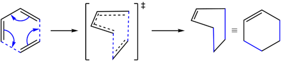Figure 25: Reaction scheme for the Diels-Alder cycloaddition of ethylene and butadiene

Reactant Structures

To determine the transition state structure, it was first necessary to optimise the reactant structures to a minimum at the AM1 level. Table 19 shows the result for the optimisation of ethylene. The HOMO and LUMO of ethylene correspond to the π-bonding orbital (symmetric) and π* antibonding orbital (antisymmetric) respectively.

Table 19

Structure

Energy

HOMO

LUMO

Energy = 16.4346461 kcal mol^-1

HOMO of ethylene (Energy = -0.38775 Hartrees) — Symmetric

LUMO of ethylene (Energy = 0.05284 Hartrees) — Antisymmetric

Table 20 summarises the results for the optimisation of s-cis butadiene. In contrast to ethylene, the HOMO is antisymmetric and the LUMO is symmetric.

Table 20

Structure

Energy

HOMO

LUMO

Energy = 30.6206993 kcal mol^-1

HOMO of butadiene (Energy = -0.34382 Hartrees) — Antisymmetric

LUMO of butadiene (Energy = 0.01708 Hartrees) — Symmetric

(One thing to watch out for is this true cis conformer (0º dihedral angle) is not a true minimum. You can perform a frequency calculation to confirm this Tam10 (talk) 14:03, 23 February 2016 (UTC))

Transition State Structure

The optimised reactant structures were copied and arranged with the ethylene fragment positioned underneath the terminal carbons of the diene, as shown in Table 21. With reference to the numbering scheme in this table, the C1-C7 and C4-C14 distances were initially set to 2.2 Å as this proved successful in the previous transition state optimisations. The optimisation to a TS(Berny) ultimately failed as the reactants drifted apart rather than converging to a transition state implying the starting distance were too long. The distances were shortened to 2.1 Å and the optimisation repeated. The calculation was successful and the results are shown in Table 21. The energy of this transition state structure is calculated to be approximately 1.5 times the sum of the reactant energies.

Table 21

Input Geometries

Calculated TS Structure

Energy

Energy = 70.0645225 kcal mol^-1

Using the atom numbering scheme shown in Table 21, the key bond lengths and angles for the input and transition state structures have been summarised in Table 22. Comparing the two geometries reveals that the distances between the carbons that form the new σ bonds (C1-C7 and C4-C14) have effectively stayed at 2.1 Å, whereas the angle of the diene relative to ethylene (C4-C14-C12) has become more obtuse and reached almost 100 °. This distance is shorter than the sum of the van der Waals radii of two carbon atoms (1.7 Å) ^[24], however it is longer than a typical C-C single bond and so it can be inferred there is some bonding interaction present.

As mentioned previously, typical C-C single and double bond lengths are 1.54 Å and 1.34 Å respectively ^[15]. All other C-C bond distances have converged to around 1.38 Å in the transition state, which is between a single and double bond and implies some delocalisation of the 6π electrons involved in the cycloaddition. The sp² C=C bonds in the reactants (C1-C4, C7-C10 and C12-C14) have lengthened and the sp³ C-C bond (C10-C12) has shortened to reach the transition state. This is as expected since in the cycloaddition, the existing C=C bonds are broken and a C=C is formed where the C-C backbone of the diene used to be (C10-C12). Interestingly, in the input structure, the C10-C12 bond length is 0.1 Å shorter than the typical C-C bond length. This is likely a result of the conjugation of the double bonds in the diene (π_C=C→π*_C=C periplanar).

Table 22
	C1-C7 Distance / Å	C4-C14 Distance / Å	C1-C4 Distance / Å	C7-C10 Distance / Å	C12-C14 Distance / Å	C10-C12 Distance / Å	C4-C14-C12 Angle / °
Input Structure	2.1	2.1	1.326	1.3351	1.3351	1.4495	78.9966
Transition State	2.1179	2.12	1.3829	1.3819	1.3819	1.3975	99.3683

Frequency Analysis

The structure obtained was confirmed to be a transition state by the presence of a single imaginary frequency (Figure 26). Figure 27 is an animation of this frequency found at -956.50 cm^-1 and is shown to be the one corresponding to the cycloaddition. From Figure 27 it can be seen that there is synchronous formation of the two new σ bonds. Furthermore, the animation beautifully shows the simultaneous stretching of the all the C=C bonds as they lengthen to single bonds and the shortening of the C-C bond of the diene as a double bond begins to form. This result supports the fact that the cycloaddition occurs via a concerted mechanism. Figure 28 illustrates the first positive ('real') vibration of the transition state found at 147 cm^-1. This is shown to be an asynchronous wagging of the ethylene fragment.

Figure 26: List of vibration frequency
Figure 27: Animation of the imaginary vibration (-956.50 cm^-1) for the ethylene + butadiene cycloaddition TS (expand to view)
Figure 28: Animation of the vibration with smallest positive frequency, mode #2 in Figure 26 (expand to view)

Molecular Orbitals of the Transition State

Figures 29 and 30 show the HOMO and LUMO of the transition state structure respectively. From comparison of the HOMO with the molecular orbitals of the reactants (shown in tables 19 and 20), it is evident this orbital has resulted from the interaction of the HOMO of butadiene with the LUMO of ethylene. Both these orbitals are antisymmetric and consequently the HOMO of the transition state is antisymmetric. Furthermore, the symmetric LUMO of the transition state is deduced to be formed from the butadiene LUMO and the ethylene HOMO, both of which are symmetric.

Since the energy difference between the butadiene HOMO & ethylene LUMO is smaller than the butadiene LUMO & ethylene HOMO (0.39666 Hartrees vs. 0.40483 Hartrees respectively), this cycloaddition is confirmed to a be a normal electron demand Diels-Alder.

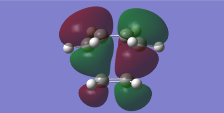Figure 29: HOMO of the transition state (Energy = -0.32393 Hartrees) — Antisymmetric
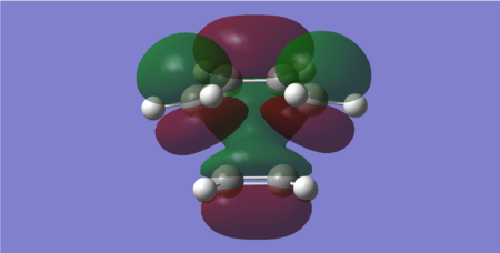Figure 30: LUMO of the transition state (Energy = 0.02316 Hartrees) — Symmetric

Intrinsic Reaction Coordinate

An IRC calculation was run on the transition state structure. The IRC was calculated in both directions for 100 steps with the force constants calculated always. Figure 31 displays the curves corresponding to the IRC animation in figure 32. The latter figure shows the animation starting with the cyclohexene structure and so the IRC corresponds to the reverse reaction; breaking of a cyclohexene ring to butadiene and ethylene. The cyclohexene ring deforms to the transition state structure (the maxima in the Total Energy along IRC graph of figure 31) and eventually breaks apart into the diene and alkene which drift apart.

The Total Energy along IRC graph shows that the cyclohexene is quite lower in energy than the diene + dienophile indicating that this structure is thermodynamically favoured. This graph also shows that the diene + dienophile are closer in energy to the transition state than cyclohexene and so it can be concluded the cycloaddition has an early transition state. Hammond's postulate states that "If two states, as, for example, a transition state and an unstable intermediate, occur consecutively during a reaction process and have nearly the same energy content, their interconversion will involve only a small reorganization of the molecular structures." ^[25]. From this it can be inferred that the transition state is more similar in structure to the diene and dienophile than the cyclohexene ring.

Figure 31: IRC curves for the ethylene + butadiene cycloaddition TS
Figure 32: Animation of the IRC (expand to view)

The starting structure from the IRC calculation (i.e. the cyclohexene ring) was copied and an opt+freq calculation to a minimum was run at the AM1 level. The results are shown in the table below and show a boat-like ring structure (C_s point group). The frequency calculation showed this structure to have an imaginary frequency which implies it is not a stable structure, but rather a transition state. The imaginary vibration, shown in Table 23, is revealed to be a twisting of two adjacent CH₂ groups, implying the structure is actually a transition state between two conformations where these methylene groups are staggered.

Table 23

Calculated Structure

Energy

Imaginary Vibration

Energy = -6.90013330 kcal mol^-1

Animation of the imaginary vibration at -54.51 cm^-1

(Be careful when quoting energies as it's fairly meaningless to convert an absolute energy into kJ/mol or kcal/mol unless they're relative to something Tam10 (talk) 14:03, 23 February 2016 (UTC))

TS(QST2) Method

To confirm whether the results from the TS(Berny) optimisation were valid, the TS(QST2) method was employed. This required the optimisation (to a minimum) of the cyclohexene product from scratch. The resulting structure and its energy at the AM1 level are shown in Table 24. This structure has a C₂ point group and is approximately 3 kcal mol^-1 lower in energy than the structure in table 23.

Table 24

Calculated Structure

Energy

Energy = -10.1624742 kcal mol^-1

Using the butadiene + ethylene geometry at 2.1 Å as the reactant and the optimised cyclohexene structure above as the product, the TS(QST2) optimisation was run. Figure 33 shows the atom labelling scheme used for this calculation. The results have not been shown in this report since they gave virtually identical results to those obtained from the TS(Berny) optimisation. The .log files have been included for reference.

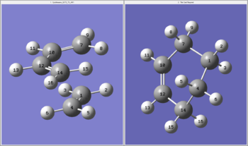Figure 33: Molecular labelling scheme used for the TS(QST2) calculation

Solution to the 'Problem'

The solution to obtaining a local minimum structure for the cyclohexene ring was to run the opt+freq calculation to a minimum with the force constant calculated once. This ensured the calculated structure was in fact a minimum since the calculation would self-check by computing the second derivative of the PES and confirming it is a positive value. Table 25 shows the structure and its energy after using this calculation method on the cyclohexene ring outputted from the IRC after TS(QST2) optimisation. Clearly the cyclohexene structure is identical to that calculated from scratch (table 24).

Table 25

Calculated Structure

Energy

Energy = -10.1624742 kcal mol^-1

Maleic Anhydride + Cyclohexa-1,3-diene Cycloaddition

The second cycloaddition studied was that of maleic anhydride and cyclohexa-1,3-diene (henceforth referred to as "cyclohexadiene"). Maleic anhydride is a common dienophile made electron-deficient by the electron withdrawing carbonyl groups which would be expected to react readily in a normal electron demand Diels-Alder. Cyclohexadiene is also a useful diene for the cycloaddition since the 6-membered ring 'locks' the double bonds in the s-cis conformation (rotation to the s-trans conformation would be too high energy a transition to occur).

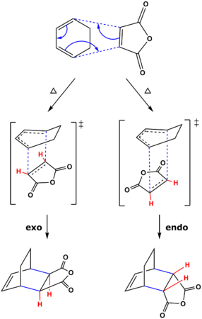Figure 34: Reaction scheme for the Diels Alder cycloaddition of maleic anhydride and cyclohexadiene

In contrast to the prototypical Diels-Alder, this reaction has the extra question of stereoselectivity. Figure 34 shows the cycloaddition and the two diastereomeric products possible; exo-bicyclo[2.2.2]oct-5-ene-2,3-dicarboxylic acid anhydride (the exo-adduct, bottom left) and endo-bicyclo[2.2.2]oct-5-ene-2,3-dicarboxylic acid anhydride (the endo-adduct, bottom right). The new C-C σ bonds formed are shown in blue and the vinyl hydrogens of maleic anhydride are shown in red. When the approach trajectory of maleic anhydride results in the vinyl protons pointing 'back' (i.e. underneath the diene backbone), the exo-adduct is formed. These protons point 'down' in the product and are trans/antiperiplanar to the CH₂-CH₂ bridge. The opposite conditions result in the endo-adduct forming. The vinyl protons point 'forward' (i.e. the carbonyls are now below the diene backbone) in the transition state and consequently point 'up' in the product.

It is often found that the thermodynamic product of a Diels-Alder cycloaddition is the exo-adduct, however the endo-adduct is found to be the major product. This selectivity towards the kinetic product was originally proposed to be due to favourable secondary orbital interactions in the endo transition state by Woodward and Hoffmann ^[26]. A secondary orbital interaction involves the two electron interaction between orbitals not directly involved in the breakage/formation of σ bonds ^[27].

Reactant Structures

The TS(QST2) method was initially chosen to locate both the exo and endo transition states. In both cases, the starting reactants are required for the calculation and so they were optimised at the AM1 level. Table 26 shows the result for maleic anhydride and table 27 the result for cyclohexadiene. The symmetry of the frontier molecular orbitals for these structures are found to be identical to the corresponding diene and dienophile of the prototypical Diels-Alder.

Table 26 shows that the carbonyl oxygen atoms make some significant contribution to both the HOMO and LUMO of maleic anhydride, though the largest contribution still comes from the π bond. The HOMO of cyclohexadiene (Table 27) shows there is some orbital contribution at the methylene groups. This is quite small compared to the contribution from the double bonds and was consequently ignored when assigning the symmetry.

Table 26

Structure

Energy

HOMO

LUMO

Energy = -76.44584344 kcal mol^-1

HOMO of maleic anhydride (Energy = -0.44187 Hartrees) — Symmetric

LUMO of maleic anhydride (Energy = -0.05949 Hartrees) — Antisymmetric

Table 27

Structure

Energy

HOMO

LUMO

Energy = 17.389100726 kcal mol^-1

HOMO of cyclohexadiene (Energy = -0.32194 Hartrees) — Antisymmetric

LUMO of cyclohexadiene (Energy = 0.01680 Hartrees) — Symmetric

Exo Transition State

Exo-Adduct Optimisation

The exo-adduct was optimised to a minimum and confirmed to have only positive vibrational frequencies by a frequency calculation. The structure and its energy are shown in Table 28 below.

Table 28

Structure

Energy

Energy = -100.344634714 kcal mol^-1

TS(QST2) Optimisation

Using the optimised reactant and exo-adduct structures, a TS(QST2) calculation was run. The reactants were positioned in the correct orientation with a separation of 2.1 Å and numbered according to the image shown in Table 29. The calculated transition state structure and its energy is also shown in this table (point group = C_s). The presence of a single imaginary frequency at -812.11 cm^-1, animated in Figure 35, confirmed this structure was in fact a transition state. This vibration again corresponds to the synchronous C-C bond formation of the cycloaddition.

Table 29

Input Geometries

Calculated Structure

Energy

Input geometries for the TS(QST2) optimisation for the exo product

Energy = -31.6389403105 kcal mol^-1

IRC Calculation

An IRC calculation in both directions with the force constant calculated 'always' was run on the exo transition state and the results shown in figures 36 and 37. It was necessary to change the Recorrect Steps option from Default to Never for the calculation to work. The IRC begins with the reactants drifting closer to each other, forming the transition state and subsequently the exo-adduct. Once again an early transition state is exhibited (see the Total Energy along IRC graph in Figure 36). From Figure 37 the structural changes are evident, most notably the change in angle of the methylene groups with respect to the diene as they gradually become the bridging groups in the exo-adduct.

Figure 35: Animation of the imaginary vibration for the exo TS (expand to view)
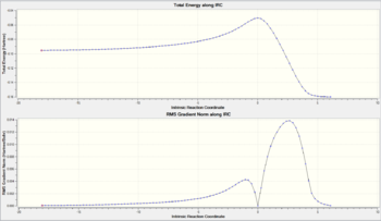Figure 36: IRC curves for the exo TS
Figure 37: Animation of the IRC for the exo TS (expand to view)

Geometry Comparison

Table 30 collates and compares the geometries of the optimised reactants (cyclohexadiene + maleic anhydride), transition state and the optimised exo-adduct using the numbering scheme shown in Table 29. The trends in the data shown in the table below are clear. For example, the C4-C6 bond starts as the double bond in maleic anhydride with a bond length typical of a C=C bond. This lengths to 1.4 Å in the transition state, a length that is virtually identical to the other C-C bond lengths for carbons that form the new cyclohexene ring. The C4-C6 bond then reaches 1.54 Å in the product, characteristic of a single bond. The bond lengths in the transition state are closer in value to the reactants than the product and this is consistent with it being an early transition state. A C4-C16-C18 angle of 92.7 °, corresponding to the angle between the diene and dienophile, is found for the transition state (c.f. 99.4 ° for the prototypical reaction).

The C13-C16-C18-C20 and H12-C10-C13-H15 dihedral angles relate to the change in geometry experience by the methylene groups. The former angle is approximately 2 ° in cyclohexadiene meaning the ring is almost flat. The latter angle is non-zero so that an eclipsed conformation is avoided. This C13-C16-C18-C20 angle sharply rises to 35 ° in the transition state while the H12-C10-C13-H15 dihedral angle goes to 0 ° as the methylene groups 'bend up' and become eclipsed. The former angle is almost 60 ° in the product indicating a gauche relationship between the C=C double bond and the bridge with respect to the C16-C18 bond.

Table 30
	C4-C16 Distance / Å	C6-C22 Distance / Å	C4-C6 Distance / Å	C16-C18 Distance / Å	C18-C20 Distance / Å	C20-C22 Distance / Å	C4-C16-C18 Angle / °	C13-C16-C18-C20 Dihedral / °	H12-C10-C13-H15 Dihedral / °
Reactants	—	—	1.3486	1.3428	1.4495	1.3428	—	1.6591	26.8021
Transition State	2.1704	2.1705	1.4101	1.3944	1.3968	1.3944	92.7369	34.3572	0.0273
Exo-adduct	1.5362	1.5361	1.5492	1.5043	1.3441	1.5043	106.6468	57.5996	0.0118

With the transition state located by the TS(QST2) method, the TS(Berny) method was attempted using the same input geometries shown in Table 29. Multiple attempts were made with varying C4-C16 distances, however all failed to converge. With the transition state in mind, the geometry of the cyclohexadiene molecule was altered such that the methylene groups 'bend up' (C13-C16-C18-C20 and C10-C22-C20-C18 angles = 30 °) and this resulted in the calculation converging successfully. This series of computations highlights the importance of providing a reasonable guess of the transition state as the input to achieve a convergence. For the prototypical reaction, simply positioning the diene and dienophile was sufficient, however, for this system, some geometry alterations were required.

Molecular Orbitals of the Exo TS

Figures 38–42, below, show orbitals of interest for the exo transition state, including the HOMO and LUMO. Both the HOMO and LUMO orbitals seem to result from the interaction of the maleic anhydride LUMO with the cyclohexadiene HOMO. The exo HOMO is a bonding interaction of these two frontier orbitals, whereas the exo LUMO is the antibonding combination. For this reaction, it seems the exo LUMO +1 is the orbital corresponding to the interaction of the maleic anhydride HOMO and cyclohexadiene LUMO. The maleic anhydride HOMO also appears to contribute to the exo HOMO -1. The exo LUMO +2 resembles the maleic anhydride LUMO +1 and cyclohexadiene LUMO +1 (both antisymmetric). Importantly, no secondary orbital interactions between the carbonyl and the diene have been exhibited in any of these orbitals, consistent with what is theoretically expected. This is likely because the carbonyls point 'away' from the diene in the exo transition state and so the relatively large spatial separation means no significant orbital overlap occurs.

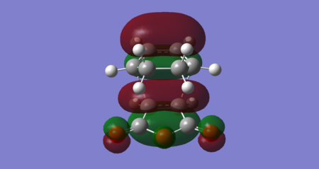Figure 38: Exo HOMO -1 (Energy = -0.36670 Hartrees) — Symmetric
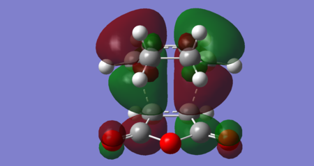Figure 39: Exo HOMO (Energy = -0.34274 Hartrees) — Antisymmetric
Figure 40: Exo LUMO (Energy = -0.04046 Hartrees) — Antisymmetric
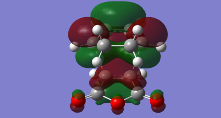Figure 41: Exo LUMO +1 (Energy = -0.02012 Hartrees) — Symmetric
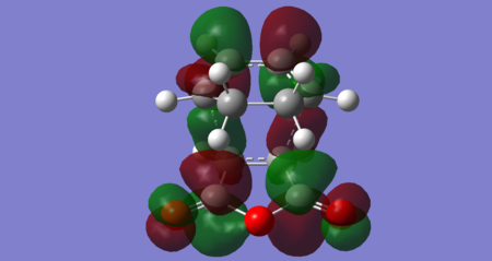Figure 42: Exo LUMO +2 (Energy = 0.03385 Hartrees) — Antisymmetric

Endo Transition State

Endo-Adduct Optimisation

The endo-adduct was optimised to a minimum and shown to have only positive frequencies by a frequency calculation. Table 31, below, shows the resulting structure and its energy.

Table 31

Structure

Energy

Energy = -100.508408 kcal mol^-1

TS(QST2) Optimisation

To obtain the endo product, the reactants were orientation as shown in Table 32 and, using the optimised endo-adduct, the the endo transition state was found using the TS(QST2) method. The results are shown below. An imaginary frequency at -805.88 cm^-1 was obtained and shown to correspond to the synchronous cycloaddition (Figure 43).

Table 32

Input Geometries

Calculated Structure

Energy

Input geometries for the TS(QST2) optimisation for the endo product

Energy = -32.3174100 kcal mol^-1

IRC Calculation

The results of the IRC for the endo transition state in both directions are shown in figures 44 and 45. As with the exo transition state, the Recorrect Steps option was changed to Never. The IRC animation (Figure 45) starts 'earlier' in the reaction coordinate than the corresponding animation for the exo transition state (Figure 37) and so the conformational change of the methylene groups from 'almost eclipsed' to eclipsed is observable. Once again, an early transition state is exhibited and the cycloaddition is shown to be concerted.

Figure 43: Animation of the imaginary vibration for the endo TS (expand to view)
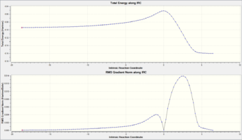Figure 44: IRC curves for the endo TS
Figure 45: Animation of the IRC for the endo TS (expand to view)

Geometry Comparison

Using the numbering scheme shown in Table 32, the geometries of the reactants, the endo transition state and the endo-adduct product have been compared in Table 33. The parameters shown are equivalent to those in Table 30. The changes in geometry observed for the exo case are also observed for the endo case, so for a detailed analysis, see the Exo Transition State - Geometry Comparison section.

Table 33
	C4-C20 Distance / Å	C6-C12 Distance / Å	C4-C6 Distance / Å	C20-C22 Distance / Å	C10-C22 Distance / Å	C10-C12 Distance / Å	C4-C20-C22 Angle / °	C17-C20-C22-C10 Dihedral / °	H16-C14-C17-H19 Dihedral / °
Reactants	—	—	1.3486	1.3428	1.4495	1.3428	—	1.6591	26.8021
Transition State	2.1616	2.1631	1.4085	1.393	1.3973	1.393	96.6275	33.5587	0.7058
Endo-adduct	1.5357	1.5358	1.5485	1.5028	1.344	1.5027	108.6386	57.6008	0.0334

Molecular Orbitals of the Endo TS

The molecular orbitals from HOMO-1 up to LUMO +2 have been shown in figures 46–50. The reactant orbitals contributing to these MOs are the same as the equivalent orbitals in the exo transition state. For example, the endo HOMO is the bonding combination of the maleic anhydride LUMO and cyclohexadiene HOMO.

The key difference between the endo and exo transition states is found for the LUMO +2 orbital. Both contain a bonding interaction between the diene LUMO +1 and dienophile LUMO +1 at the carbons that form the new σ bonds in the cycloaddition, however there is an additional secondary orbital interaction exhibited in the endo transition state. This is the bonding interaction between the diene LUMO +1 at the carbons where a double bond forms in the cycloaddition (C10-C22) and the dienophile LUMO +1 at the carbonyl carbons (which resembles the π* C=O orbital). The interaction has arisen in the endo transition state since the diene backbone and the carbonyls are in close proximity and have the correct orbital symmetry. The former condition is not met in the exo transition state.

Figure 46: Endo transition state HOMO -1 (Energy = -0.36843 Hartrees) — Symmetric
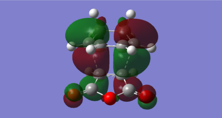Figure 47: Endo transition state HOMO (Energy = -0.34505 Hartrees) — Antisymmetric
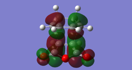Figure 48: Endo transition state LUMO (Energy = -0.03565 Hartrees) — Antisymmetric
Figure 49: Endo transition state LUMO +1 (Energy = -0.02016 Hartrees) — Symmetric
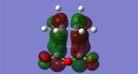Figure 50: Endo transition state LUMO +2 (Energy = 0.02867 Hartrees) — Antisymmetric

Exo vs. Endo Comparison

Activation Energies

The key thermodynamic parameters for all species in the maleic anhydride + cyclohexadiene cycloaddition have been tabulated below (Table 34). The energy values for Reactants have been calculated as a sum of the values for isolated maleic anhydride and cyclohexadiene. As expected, the energy becomes more positive going from left to right in the table due to the additional contributions to the energy (as discussed previously).

Table 34
	Electronic Energy / Hartrees	Sum of Electronic and Zero-Point Energies (0 K) / Hartrees	Sum of Electronic and Thermal Energies (298.15 K) / Hartrees
Maleic Anhydride	-0.12182418	-0.063346	-0.058192
Cyclohexadiene	0.02771129	0.152502	0.157726
Reactants	-0.09411289	0.089156	0.099534
Exo TS	-0.05041985	0.134881	0.144882
Endo TS	-0.05150106	0.133494	0.143684
Exo-adduct	-0.15990932	0.031702	0.040680
Endo-adduct	-0.16017031	0.031464	0.040462

Using the values from Table 34, key energy differences for the exo and endo cyclisations have been calculated and tabulated in Table 35. The Energy Difference at 0 K and the Energy Difference at 298.15 K have been calculated using Sum[s] of Electronic and Zero-Point Energies (0 K) and Sum[s] of Electronic and Thermal Energies (298.15 K) respectively.

Table 35
	Energy Difference at 0 K / kcal mol^-1	Energy Difference at 298.15 K / kcal mol^-1
ΔE^‡_exo	28.69	28.46
ΔE^‡_endo	27.82	27.70
ΔE_{rxn, exo}	-36.05	-36.93
ΔE_{rxn, endo}	-36.20	-37.07

ΔE^‡ is defined as the energy difference between a transition state and the reactants. This gives the activation energy for the reaction, a kinetic parameter. Firstly, it can be seen that the activation energy is smaller at 298.15 K than at 0 K, an observation also made in the Cope rearrangement case. In contrast to the Cope rearrangement, the difference much smaller (less than 0.3 kcal mol^-1 here), indicating a smaller temperature dependence of the activation energy for this Diels-Alder cycloaddition. Importantly, ΔE^‡_exo is shown to be approximately 1 kcal mol^-1 greater than ΔE^‡_endo , revealing that there is a larger kinetic barrier to the exo-adduct. From these values, the endo-adduct is confirmed to be the kinetically preferred product.

It should be noted that literature values for the activation energy of this cycloaddition has been reported as 11 kcal mol^-1 in dichloromethane ^[28]. This difference to the computed activation energies here are likely due to the approximations made in the AM1 method. An optimisation at the B3LYP/6-31G* level is required for more accurate values, however the AM1 method is sufficient to make a valid conclusion about the relative energies of the exo and endo transition states.

ΔE_rxn is defined as the energy difference between the product (exo- or endo-adduct) and the reactants. Since the energy for the reactants was calculated simply as a sum, ΔE_rxn corresponds to the forming the adduct from the reactants starting at infinite separation. ΔE_rxn is a thermodynamic parameter and can therefore be used to evaluate the relative stabilities of the exo- and endo-adducts. Both ΔE_{rxn, exo} and ΔE_{rxn, endo} are negative and so the cycloaddition is thermodynamically favoured. From comparison of these two parameters, the endo-adduct is shown to be thermodynamically more stable than the exo-adduct (ΔE_{rxn, endo} is more negative).

Analysis of Strain

Secondary orbital interactions have been shown to stabilise the endo transition state thus making the endo-adduct the kinetic product. Since these orbital interactions are no longer present in the endo-adduct itself to make it the thermodynamic product, it can be deduced that either the endo-adduct is favoured or the exo-adduct is disfavoured due to the geometry.

Both adducts were temporarily relabelled according to Figure 51 for this section to allow for comparison. (The numbering here does not match that in the log files.)

Since both adducts consist of the same three 6-membered rings (C4-C6-C16-C14-C12-C10, C10-C12-C14-C16-C18-C21 and C4-C6-C16-C18-C21-C10) and the same 5-membered ring (O1-C2-C4-C5-C8), ring strains were disregarded. They do, however, differ in their connectivity at C4 & C6 and so the angle strain here was considered, but no significant difference was found.

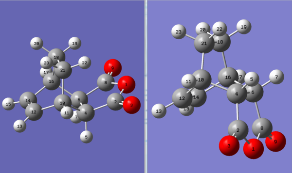Figure 51:Labelling scheme for the exo-adduct (left) and endo-adduct (right)

The steric strain between the CH₂-CH₂ bridge and the anhydride moiety was examined. Table 36 shows the interatomic distances between atoms that could potentially clash with C21 and H22 of the bridge. The van der Waals radii of oxygen, carbon and hydrogen are 1.52 Å, 1.7 Å and 1.2 Å respectively ^[24] and so the sum of these radii are as follows:

O-H = 2.74 Å
O-C = 3.24 Å
C-H = 2.9 Å
C-C = 3.4 Å
H-H = 2.4 Å

Table 36
	O1-H22 Distance / Å	C2-H22 Distance / Å	O3-H22 Distance / Å	C4-H22 Distance / Å	H5-H22 Distance / Å	O1-C21 Distance / Å	C2-C21 Distance / Å	O3-C21 Distance / Å	C4-C21 Distance / Å	H5-C21 Distance / Å
Exo-adduct	3.06628	2.56588	2.93704	2.74112	3.75580	3.50360	2.94291	3.57527	2.49517	3.47592
Endo-adduct	5.06933	4.13104	4.83921	2.69406	2.45073	4.67305	3.84704	4.63135	2.46327	2.70658

Firstly, the oxygen atoms of the anhydride moiety are not observed to sterically clash with the bridge. The C4-H22 and C4-C21 distances are seen to be shorter than the sum of the van der Waals radii for C-H and C-C respectively and though they technically clash, this can be ignored since the effect is present in both adducts. The H5-C21 distance is also seen to be short in the endo-adduct, however this is not as significant when compared to the C2-H22 distance in the exo-adduct. The dominant factor resulting in the exo-adduct having greater steric strain than the endo-adduct is the C2-C21 distance. This distance is 2.94291 Å in the exo-adduct which is much shorter then the sum of the van der Waals radii of two carbon atoms. This steric strain energetically disfavours the exo-adduct and means the thermodynamic product is the endo-adduct.

(Good to see the inclusion of the endo and exo products Tam10 (talk) 14:03, 23 February 2016 (UTC))

Conclusion

The Cope rearrangement of 1,5-hexadiene was studied at the HF/3-21G and B3LYP/6-31G* levels. Various conformations of 1,5-hexadiene were analysed, but the most stable conformation was determined to be the Gauche 3 conformer due to a favourable bonding interaction between the π bonding orbitals of the two C=C bonds. The chair and boat transition states for the rearrangement were located by various methods and, by comparison of activation energies, the energy of the former shown to be lower.

Two normal electron demand Diels-Alder cycloadditions – ethylene + butadiene and maleic anhydride + cyclohexa-1,3-diene – were studied at the AM1 level and revealed to have early transition states through intrinsic reaction coordinate calculations. The molecular orbitals of the exo and endo transition states for the latter reaction were computed and evidence of secondary orbital interactions for the endo transition state found. Through comparison of the energies, the endo-adduct was determined to be both the kinetic and thermodynamic product of the maleic anhydride + cyclohexa-1,3-diene cycloaddition.

References

↑ ^1.0 ^1.1 M. J. Bearpark, 'Lecture 3: Calculating Energies: Methods/Basis Sets', Quantum Mechanics 3/Core 3^rd Year Computational Chemistry Laboratory, 19/10/2015, Imperial College London, 2015.
↑ Hartree-Fock Method, https://en.wikipedia.org/wiki/Hartree%E2%80%93Fock_method, accessed 06/02/16.
↑ J. Tirado-Rives and W. L. Jorgensen, J. Chem. Theory Comput., 2008, 4, 297–306. DOI:10.1021/ct700248k
↑ M. J. S. Dewar, E. G. Zoebisch, E. F. Healy and J. J. P. Stewart,J. Am. Chem. Soc., 1985, 107, 3902–3909. DOI:10.1021/ja00299a024
↑ Basis Sets, http://www.gaussian.com/g_tech/g_ur/m_basis_sets.htm, accessed 06/12/2016.
↑ M. Bearpark, F. Bernardi, M. Olivucci and M. A. Robb, J. Am. Chem. Soc., 1990, 112, 1732–1737. DOI:10.1021/ja00161a012
↑ N. L. Allinger, J. T. Fermann, W. D. Allen and H. F. Schaefer III, J. Chem. Phys., 1997, 106, 5143. DOI:10.1063/1.473993
↑ ^8.0 ^8.1 ^8.2 B. W. Gung, Z. Zhu and R. A. Fouch, J. Am. Chem. Soc., 1995, 117, 1783–1788. DOI:10.1021/ja00111a016
↑ B. G. Rocque, J. M. Gonzales and H. F. Schaefer III, Mol. Phys., 2002, 100, 441–446. DOI:10.1080/00268970110081412
↑ Y. Umezawa, S. Tsuboyama, H. Takahashi, J. Uzawa and Motohiro Nishio, Tetrahedron, 1999, 55, 10047–10056. DOI:10.1016/S0040-4020(99)00539-6
↑ ^11.0 ^11.1 G. Schultz and I. Hargittai, J. Mol. Struct., 1995, 346, 63–69. DOI:10.1016/0022-2860(94)09007-C
↑ P. Atkins and J. de Paula, Physical Chemistry, W. H. Freeman and Company, New York, 8th edn., 2006, ch. 13, pp. 454–455. ISBN: 0-7167-8759-8.
↑ ^13.0 ^13.1 J. W. Ochterski, Thermochemistry in Gaussian, 2000. Accessed 27/01/2016.
↑ ^14.0 ^14.1 D. A. Dixon and A. Komornicki, J. Phys. Chem., 1990, 94, 5630–5636. DOI:10.1021/j100377a041
↑ ^15.0 ^15.1 L. S. Bartell, J. Am. Chem. Soc., 1959, 81, 3497–3498. DOI:10.1021/ja01523a002
↑ E. Cané, A. Miani and A. Trombetti, J. Chem. Educ., 1999, 76, 1288. DOI:10.1021/ed076p1288
↑ N. Leventis, S. B. Hanna and C. Sotiriou-Leventis, J. Chem. Educ., 1997, 74, 813. DOI:10.1021/ed074p813
↑ M. J. Goldstein and M. S. Benzon, J. Am. Chem. Soc., 1972, 94, 7147–7149. DOI:10.1021/ja00775a046
↑ ^19.0 ^19.1 T.L. Cottrell, The Strengths of Chemical Bonds, Butterworths, London, 2nd edn., 1958.
↑ R. B. Woodward and R. Hoffmann, Angew. Chem. Int. Ed. (English), 1969, 8, 781–853. DOI:10.1002/anie.196907811
↑ M. V. Basilevskii, A. G. Shamov, V. A. Tikhomirov, . Am. Chem. Soc., 1977, 99, 1369–1372. DOI:10.1021/ja00447a014
↑ R. L. Lipnick and E. W. Garbisch Jr., J. Am. Chem. Soc., 1973, 95, 6370–6375. DOI:10.1021/ja00800a034
↑ A. C. Spivey, 'Lecture 2: Stereoelectronics of Ground States – Conformational Analysis', Chemistry III (Organic): An Introduction to Reaction Stereoelectronics,10/11/2015, Imperial College London, 2015.
↑ ^24.0 ^24.1 A. Bondi, J. Phys. Chem., 1964, 68, 441–451. DOI:10.1021/j100785a001
↑ G. S. Hammond, J. Am. Chem. Soc., 1955, 77, 334–338. DOI:10.1021/ja01607a027
↑ R. Hoffmann and R. B. Woodward, J. Am. Chem. Soc., 1965, 87, 4388–4389. DOI:10.1021/ja00947a033 .
↑ A. Arrieta and F. P. Cossio, J. Org. Chem., 2001, 66, 6178-6180. DOI:10.1021/jo0158478
↑ C. A. Eckert and R. A. Grieger, J. Am. Chem. Soc., 1970, 92, 7149–7153. DOI:10.1021/ja00727a021

[am-1] 1.0 ^1.1 M. J. Bearpark, 'Lecture 3: Calculating Energies: Methods/Basis Sets', Quantum Mechanics 3/Core 3^rd Year Computational Chemistry Laboratory, 19/10/2015, Imperial College London, 2015.

[2] Hartree-Fock Method, https://en.wikipedia.org/wiki/Hartree%E2%80%93Fock_method, accessed 06/02/16.

[3] J. Tirado-Rives and W. L. Jorgensen, J. Chem. Theory Comput., 2008, 4, 297–306. DOI:10.1021/ct700248k

[4] M. J. S. Dewar, E. G. Zoebisch, E. F. Healy and J. J. P. Stewart,J. Am. Chem. Soc., 1985, 107, 3902–3909. DOI:10.1021/ja00299a024

[5] Basis Sets, http://www.gaussian.com/g_tech/g_ur/m_basis_sets.htm, accessed 06/12/2016.

[6] M. Bearpark, F. Bernardi, M. Olivucci and M. A. Robb, J. Am. Chem. Soc., 1990, 112, 1732–1737. DOI:10.1021/ja00161a012

[7] N. L. Allinger, J. T. Fermann, W. D. Allen and H. F. Schaefer III, J. Chem. Phys., 1997, 106, 5143. DOI:10.1063/1.473993

[am1-8] 8.0 ^8.1 ^8.2 B. W. Gung, Z. Zhu and R. A. Fouch, J. Am. Chem. Soc., 1995, 117, 1783–1788. DOI:10.1021/ja00111a016

[am2-9] B. G. Rocque, J. M. Gonzales and H. F. Schaefer III, Mol. Phys., 2002, 100, 441–446. DOI:10.1080/00268970110081412

[10] Y. Umezawa, S. Tsuboyama, H. Takahashi, J. Uzawa and Motohiro Nishio, Tetrahedron, 1999, 55, 10047–10056. DOI:10.1016/S0040-4020(99)00539-6

[am7-11] 11.0 ^11.1 G. Schultz and I. Hargittai, J. Mol. Struct., 1995, 346, 63–69. DOI:10.1016/0022-2860(94)09007-C

[12] P. Atkins and J. de Paula, Physical Chemistry, W. H. Freeman and Company, New York, 8th edn., 2006, ch. 13, pp. 454–455. ISBN: 0-7167-8759-8.

[am3-13] 13.0 ^13.1 J. W. Ochterski, Thermochemistry in Gaussian, 2000. Accessed 27/01/2016.

[am4-14] 14.0 ^14.1 D. A. Dixon and A. Komornicki, J. Phys. Chem., 1990, 94, 5630–5636. DOI:10.1021/j100377a041

[bondl-15] 15.0 ^15.1 L. S. Bartell, J. Am. Chem. Soc., 1959, 81, 3497–3498. DOI:10.1021/ja01523a002

[16] E. Cané, A. Miani and A. Trombetti, J. Chem. Educ., 1999, 76, 1288. DOI:10.1021/ed076p1288

[am5-17] N. Leventis, S. B. Hanna and C. Sotiriou-Leventis, J. Chem. Educ., 1997, 74, 813. DOI:10.1021/ed074p813

[18] M. J. Goldstein and M. S. Benzon, J. Am. Chem. Soc., 1972, 94, 7147–7149. DOI:10.1021/ja00775a046

[bond-19] 19.0 ^19.1 T.L. Cottrell, The Strengths of Chemical Bonds, Butterworths, London, 2nd edn., 1958.

[20] R. B. Woodward and R. Hoffmann, Angew. Chem. Int. Ed. (English), 1969, 8, 781–853. DOI:10.1002/anie.196907811

[21] M. V. Basilevskii, A. G. Shamov, V. A. Tikhomirov, . Am. Chem. Soc., 1977, 99, 1369–1372. DOI:10.1021/ja00447a014

[22] R. L. Lipnick and E. W. Garbisch Jr., J. Am. Chem. Soc., 1973, 95, 6370–6375. DOI:10.1021/ja00800a034

[23] A. C. Spivey, 'Lecture 2: Stereoelectronics of Ground States – Conformational Analysis', Chemistry III (Organic): An Introduction to Reaction Stereoelectronics,10/11/2015, Imperial College London, 2015.

[vdw-24] 24.0 ^24.1 A. Bondi, J. Phys. Chem., 1964, 68, 441–451. DOI:10.1021/j100785a001

[25] G. S. Hammond, J. Am. Chem. Soc., 1955, 77, 334–338. DOI:10.1021/ja01607a027

[26] R. Hoffmann and R. B. Woodward, J. Am. Chem. Soc., 1965, 87, 4388–4389. DOI:10.1021/ja00947a033 .

[27] A. Arrieta and F. P. Cossio, J. Org. Chem., 2001, 66, 6178-6180. DOI:10.1021/jo0158478

[28] C. A. Eckert and R. A. Grieger, J. Am. Chem. Soc., 1970, 92, 7149–7153. DOI:10.1021/ja00727a021

[1]

[2]

[3]

[4]

[5]

[6]

[7]

[8]

[9]

[10]

[11]

[12]

[13]

[14]

[15]

[16]

[17]

[18]

[19]

[20]

[21]

[22]

[23]

[24]

[25]

[26]

[27]

[28]