Rep:AM4462

Introduction to Molecular Dynamics: Simulation of a Simple Liquid

Molecular Dynamics Simulation is a power tool used to model the physical movements of particles (e.g. atoms or molecules) over a given time. It also allows us to calculate thermodynamic quantities, such as the temperature, pressure and density, for the system as a whole.

This report details the use of MD simulations to model the behaviour of a simple Lennard-Jones fluids. The input scripts were created and edited on Notepad++ and run using the LAMMPS code on the Imperial High Performance Computing Systems (HPC).

Background Work

Velocity-Verlet Algorithm

Figure 1: Time vs. position graph for a simple harmonic oscillator with t = 0.1

Figure 2: Time vs. computed energy graph for a simple harmonic oscillator with t = 0.1

Figure 3: Time vs. absolute error graph with t = 0.1

Figure 4: Time vs. percentage of original energy value plot for t = 0.2

MD simulations rely on statistical physics, in particular Newton's second law of motion, given below. In words, the equation states that acceleration is the first derivative of velocity with respect to time and the second derivative of position with respect to time.

${\mathrm{F}}_i=m_i{\mathbf{a}}_i=m_i\frac{\mathrm{d}{\mathbf{v}}_i}{\mathrm{d}t}=m_i\frac{{\mathrm{d}}^2{\mathbf{x}}_i}{\mathrm{d}{t}^2}$

The Velocity-Verlet algorithm is used to numerically solve these equations by calculating in discrete timesteps rather than as a continuous function of time. (More information here.)

Using the simple 1D harmonic oscillator as an example, the Velocity-Verlet algorithm was used to calculate the position and velocity and the results compared with the classic solution for the position at time t. The classic position is given by the equation below.

$x(t)=Acos(\omega t+\varphi )$

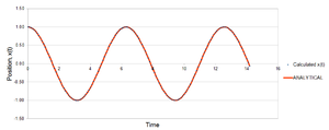
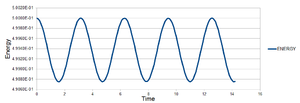
The following constants were used: t = 0.100, m = 1.0, φ = 0, A = 1.0 and ω = 1.0. Figure 1 shows how the position varies with time. It can be seen that the position oscillates regularly between ±1.00, as would be expected for a harmonic oscillator. The total energy can also be seen to fluctuate from figure 2, between $4.88\cdot 10^{-1}$ and $5.00\cdot 10^{-1}$. It would be expected that the total energy is constant for the harmonic oscillator, oscillating between kinetic and potential energy and being conserved. Since this fluctuation is very small, it can be said that the results give acceptable physical behaviour since the energy is virtually constant.

Furthermore, by visual inspection of figure 1, it seems that the simulated and classically calculated positions are in good agreement. Figure 3 reveals that as the time increases, the error between the simulated and calculated position increases, with local maxima approximately at times when x(t) = 0. The local maxima are linked by the orange trend line in this figure. There is a positive linear correlation between the time and the error. This error stems from how the Velocity-Verlet algorithm is derived. Since the algorithm is an approximation, based on a Taylor expansion, small errors in the simulated position accumulate over time resulting in the plot observed in figure 3.

The timestep value, t, was then altered such that the total energy does not vary by greater than 1 % of the original value. The critical value was found to be t = 0.200 and figure 4 demonstrates how the percentage error varies with time. This doubling of the timestep means more time is simulated for a given number of timesteps.

It is always important to monitor the total energy when numerically modelling a physical system to ensure the results are consistent with what is expected, i.e. total energy is conserved and at a constant value. This ensures that the results and conclusions which may be derived from the simulation are meaningful.

Atomic Forces

In order to calculate the forces experienced by particles in a simulation, the Lennard-Jones potential is used to determine the pairwise interactions. These pairwise potentials are summed for all pairs of particles. The following equation is the Lennard-Jones potential for just one pair of particles. In this equation, ε is the potential well depth (a measure of the strength of interaction), σ is the distance at which the potential energy is zero and $r$is the distance between the interacting particles.

$\varphi (r)=4ϵ\left[\right(\frac{\sigma }{r}{)}^{12}-\left(\frac{\sigma }{r}{)}^6\right]$

Separation, $r_0$, at which potential energy is zero

When $\varphi (r)$ = 0, $r=r_0$, hence:

$0=4ϵ\left[\right(\frac{\sigma }{r_0}{)}^{12}-\left(\frac{\sigma }{r_0}{)}^6\right]$

$0=(\frac{\sigma }{r_0}{)}^{12}-(\frac{\sigma }{r_0}{)}^6$

By rearranging this equation, the following result is obtained:

${\sigma }^6={r_0}^6$

$$\begin{gathered} \therefore \\ {r}_0=\sigma \end{gathered}$$

The force at separation $r=r_0$

The force is given by the negative derivative of the potential as shown by the equation below.

$\mathrm{F}=-\frac{\mathrm{d}\varphi (r)}{\mathrm{d}r}$

The derivative of the Lennard-Jones potential is given by the following equation, assuming є and σ are constant:

$\frac{\mathrm{d}\varphi (r)}{\mathrm{d}r}=4ϵ[-12(\frac{{\sigma }^{12}}{r^{13}})+6(\frac{{\sigma }^6}{r^7}\left)\right]$

$\frac{\mathrm{d}\varphi (r)}{\mathrm{d}r}=24ϵ\left[\right(\frac{{\sigma }^6}{r^7})-2(\frac{{\sigma }^{12}}{r^{13}}\left)\right]$

Since

$r=r_0$

and

$\sigma =r_0$

:

$\frac{\mathrm{d}\varphi (r)}{\mathrm{d}r}=24ϵ\left[\right(\frac{{r_0}^6}{{r_0}^7})-2(\frac{{r_0}^{12}}{{r_0}^{13}}\left)\right]$

$\frac{\mathrm{d}\varphi (r)}{\mathrm{d}r}=24ϵ[\frac{1}{r_0}-\frac{2}{r_0}]$

$\frac{\mathrm{d}\varphi (r)}{\mathrm{d}r}=-24ϵ\left[\frac{1}{r_0}\right]$

From the equation given for force:

$$\begin{gathered} \therefore \\ \mathrm{F}=\frac{24ϵ}{r_0} \end{gathered}$$

Calculating the equilibrium separation, $r_{eq}$

Since the equilibrium separation corresponds to the global minimum potential of the Lennard-Jones potential, we can find $r_{eq}$ by setting the derivative of the Lennard-Jones potential equation to zero. Using the derivative found in the previous section and substituting in $r=r_{eq}$:

$\frac{\mathrm{d}\varphi (r)}{\mathrm{d}r}=24ϵ\left[\right(\frac{{\sigma }^6}{{r_{eq}}^7})-2(\frac{{\sigma }^{12}}{{r_{eq}}^{13}}\left)\right]=0$

$\frac{{\sigma }^6}{{r_{eq}}^7}=2\left(\frac{{\sigma }^{12}}{{r_{eq}}^{13}}\right)$

This rearranges to:

${r_{eq}}^6=2{\sigma }^6$

$$\begin{gathered} \therefore \\ {r}_{eq}=\sqrt[6]{2} \\ \sigma \end{gathered}$$

Calculating the well depth at $r_{eq}$

$\varphi (r_{eq})=4ϵ\left[\right(\frac{\sigma }{r_{eq}}{)}^{12}-\left(\frac{\sigma }{r_{eq}}{)}^6\right]$

$$\begin{gathered} \varphi (r_{eq})=4ϵ\left[\right(\frac{\sigma }{\sqrt[6]{2} \\ \sigma }{)}^{12}-\left(\frac{\sigma }{\sqrt[6]{2} \\ \sigma }{)}^6\right] \end{gathered}$$

This simplifies to the following:

$ϵ=-\varphi (r_{eq})$

Evaluating the integrals of the Lennard-Jones Potential

$\int \varphi (r)\mathrm{d}r=4ϵ(\frac{{\sigma }^6}{5r^5}-\frac{{\sigma }^{12}}{11r^{11}})+C$

Given that $\sigma ==1.0$:

$\int \varphi (r)\mathrm{d}r=4ϵ(\frac{1}{5r^5}-\frac{1}{11r^{11}})+C$

For the following integrals, $ϵ=\sigma =1.0$. Since at $r=\mathrm{\infty }$ there is not interaction better particles, $\varphi (r)=0$:

$$\begin{gathered} \underset{2\sigma }{\overset{\mathrm{\infty }}{\int }}\varphi (r)\mathrm{d}r=-0.0248 \\ (3s.f.) \end{gathered}$$

$$\begin{gathered} \underset{2.5\sigma }{\overset{\mathrm{\infty }}{\int }}\varphi (r)\mathrm{d}r=-0.00818 \\ (3s.f.) \end{gathered}$$

$$\begin{gathered} \underset{3\sigma }{\overset{\mathrm{\infty }}{\int }}\varphi (r)\mathrm{d}r=-0.00329 \\ (3s.f.) \end{gathered}$$

These results show that as the lower boundary increases, the integral decreases in magnitude. This allows us to determine a suitable 'cut-off' distance for the Lennard-Jones potential, $r_c$, by making an appropriation that beyond $r_c$ the integral/pairwise interaction is negligible.

Periodic Boundary Conditions

Estimate for the number of water molecules in 1ml of water under standard conditions

Assuming that for water, 1 mL = 1 g:

no. of moles $$\begin{gathered} =\frac{mass}{M_r}=\frac{1}{18} \\ mol \end{gathered}$$

no. of molecules $$\begin{gathered} =\frac{N_A}{18} \\ =3.35\cdot 10^{22}(3s.f.) \end{gathered}$$

Where $N_A$ is Avogadro's Number.

Estimate for the volume of 10000 water molecules under standard conditions

10000 molecules of water $$\begin{gathered} =\frac{10000}{N_A} \\ mol \end{gathered}$$

mass $$\begin{gathered} =\frac{10000}{N_A} \\ mol\cdot 18 \\ g \\ mo{l}^{-1} \end{gathered}$$

mass $$\begin{gathered} =2.99\cdot 10^{-19} \\ \mathrm{g} \end{gathered}$$

volume $$\begin{gathered} =2.99\cdot 10^{-19} \\ \mathrm{mL} \end{gathered}$$

Consider an atom at position (0.5, 0.5, 0.5) in a cubic simulation box which runs from (0, 0, 0) to (1, 1, 1). In a single timestep, it moves along the vector (0.7, 0.6, 0.2). At what point does it end up, after the periodic boundary conditions have been applied?

(0.5, 0.5, 0.5) + (0.7, 0.6, 0.2) = (1.2, 1.1, 0.7) Since the box is limited to (1, 1, 1), (1.2, 1.1, 0.7) is equivalent to (0.2, 0.1, 0.7). The result comes from the fact that in a simulation, infinite space cannot be simulated. To work around this, boundary conditions are set. Since a particle cannot exist outside the box, a particle on vector that leads to a position outside the box, like in this question, will appear on the 'other side' of the box as if it came from another simulation box.

Reduced Units

The Lennard-Jones parameters for argon are σ = 0.34 nm, є/K_B = 120 K. If the LJ cutoff is r* = 3.2, what is it in real units?

$r^{*}=\frac{r}{\sigma }$

$$\begin{gathered} r=3.2\cdot 0.34 \\ nm \end{gathered}$$

$$\begin{gathered} r=1.1 \\ nm \\ (3s.f.) \end{gathered}$$

What is the well depth in kJ mol^-1?

$$\begin{gathered} ϵ=120 \\ \mathrm{K}\cdot k_B \end{gathered}$$

$$\begin{gathered} ϵ=1.7\cdot 10^{-21}\mathrm{J} \\ (2s.f.) \end{gathered}$$

Multiplication by Avogadro's Number gives:

$$\begin{gathered} ϵ=1.0 \\ \mathrm{kJ} \\ mo{l}^{-1} \\ (2s.f.) \end{gathered}$$

What is the reduced temperature T* = 1.5 in real units?

$T^{*}=\frac{k_{B}T}{ϵ}$

$$\begin{gathered} T^{*}=1.5\cdot 120 \\ \mathrm{K} \end{gathered}$$

$$\begin{gathered} T=180 \\ \mathrm{K} \end{gathered}$$

Outputs of the First Set of Simulations

Creating the Simulation Box

Figure 5: Simple cubic lattice

When creating a simulation, the issue of generating starting positions for the particles arises. Giving atoms random starting coordinates is unsuitable because there is always a possibility that particles may overlap each other. Of course, this is not physically possible and so the simulation would not be suitable. The solution is to create a lattice and position one atom per lattice point. In the input script the following command is given:

lattice sc 0.8
region box block 0 10 0 10 0 10
create_box 1 box
create_atoms 1 box
The first line forms a simple cubic (sc) lattice with number density of 0.8 units. The second line defines a region called 'box' which extends 10 lattice spacings in all 3 dimensions from an origin point. The third line creates the desired 'box' using just '1' atom type. The create_atoms function then creates the atoms of type '1' and fills every lattice point in the 'box' with atoms. Since the 'box' contains 1000 unit cells (10*10*10), 1000 atoms are created.

Figure 6: Face-centred cubic lattice

Proof of the number density for SC

There is one lattice point per SC unit cell and given that the number density is the number of lattice points per unit volume, $\frac{N}{V}$,the volume is given by 1/0.8 = 1.25. Taking the cube root of this gives the length of the unit cell (i.e. lattice spacing) which is 1.07722 (5 d.p.). This is exactly the lattice spacing given in the output file, hence proving that 0.8 is indeed the number density.

Consider instead a face-centred cubic lattice with a lattice point number density of 1.2

In an FFC lattice, there are 4 lattice points per unit cell since the corner points contribute 1/8 th of a lattice point while those on the face contribute half a lattice point each. Applying the same method as in the section above, the lattice spacing is calculated to be 1.49380 (5 d.p.). Since each FCC unit cell contains 4 lattice points, the create_atoms command would create 4000 atoms (4*10*10*10).

Setting the properties of atoms

In the previous section, we defined the initial position of each atom, $x_i(0)$, in the simulation and now we must define the physical properties of these atoms. The mass and Lennard-Jones interactions are defined by the code below.

mass 1 1.0
pair_style lj/cut 3.0
pair_coeff * * 1.0 1.0

The first line defines the mass of all type '1' atoms to equal '1.0'. The pair_style command is used to define the type of pairwise interactions that will be computed. In this case we are interested in the standard '12/6' Lennard-Jones potential ('lj'). The lj/cut style computed the LJ potential with a cut-off $r_c$ = 3.0 (as previously mentioned). The pairwise force field coefficients are also defined using the pair_coeff command. In line 3 above, asterisks (known as 'wildcards') have been used to represent all atom types, hence the coefficients for every pair of atoms has been defined by this line. In the input script, since we only deal with atom type '1', these asterisks are replaced by the number '1'.

The initial velocities, $v_i(0)$, for all the atoms is also defined by a line of command see later. Given that we are defining both the initial position and velocity for each each atom, we will use the Velocity-Verlet Algorithm for the simulation.

Running the simulation

Another important quantity that must be defined for the simulation is the timestep. The following code was used in the input script.

variable timestep equal 0.001
variable n_steps equal floor(100/${timestep})
timestep ${timestep}
run ${n_steps}

The variable command is used to define a new variable which is stored in the memory and can be recalled later in the script. For example, the first line creates a new variable called 'timestep' and gives it a fixed value of 0.001 (i.e. fixed within the scope of a single simulation). This value can be altered between simulations as desired. This variable is later referred to in lines 2 and 3 using the ${*} notation. The floor command is used in line 2 to round down the given value of '100/${timestep}' to the nearest integer. The 3rd line is used to define the timestep to be used in the simulation and finally the last line runs the simulations for a given number of timesteps (values defined by 'n_steps').

This string of code is useful as it ensure that no matter what timestep is chosen, the same length of time is simulated, useful for comparing the effect of timestep on the simulation results. For example if timestep = 0.001, run = 100000 and so 100 time units is simulated. If timestep = 0.002, run = 50000 and so 100 time units is also simulated.

Checking equilibration

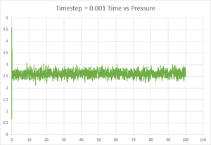
An input script that incorporated the commands discussed previously was run (timestep = 0.001). The key thermodynamic quantities that were outputted are plotted in figures 7, 8 and 9 below. They show that after a very short time, the system equilibrates, which some fluctuations around particular values of total energy, temperature and pressure. After just 0.3 time units, the system is seen to equilibrate to an average total energy of approximately -3.184 reduced units, an average temperature of -1.256 units and an average pressure of 2.615 units (all to 4 d.p.).

Figure 7: Time vs. total energy graph for t = 0.001

Figure 8: Time vs. temperature graph for t = 0.001

Figure 9: Time vs pressure graph for t = 0.001

Figure 10: Time vs. total energy graph for various timestep values

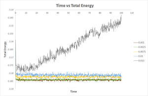
A set of simulations was run in order to investigate the effect of timestep on the computed total energy as function of simulated time. 5 values of timestep were used between 0.001 and 0.015. The results are shown in the graph above (figure 10). It can be seen from figure 10 that as the timestep value is increased, the total energy value computed systematically increases (becomes more positive). The result obtained for timestep = 0.015 is exceptionally bad since the total energy is actually seen to increase over the course of the simulation after an equilibration period. The large timestep results in a larger error because the simulation is effectivel 'monitored' less closely/regularly and so the results are less accurate. This is because properties of the system between these large timesteps is not monitored. The lowest energy is obtained for the shortest timestep, however there is minor difference between the computed energy for t = 0.001 and t = 0.0025. It is therefore acceptable to proceed using t = 0.0025 since it provides a suitably accurate result while allowing a longer period of time to be simulated.

Running simulations under specific conditions

Temperature and Pressure Control

Figure 11: Temperature vs. density graph for data at two pressures, with standard error bars plotted for the simulation data

The simulations in the previous section were run under NVE conditions (constant number of atoms, volume and energy). In this section, the model fluid being simulated will be 'taken to' NVE conditions and then run under NpT conditions (constant number of atoms, pressure and temperature). In the previous section, the average computed pressure at equilibrium was found to be

$P=2.6$

(to 1 d.p.). Simulations at 5 different temperatures above the critical temperature of

${\mathrm{T}}^{*}=1.5$

were run. This was done for

$P=2.6$

and

$P=3.0$

. therefore totaling 10 simulations. The computed density for each simulation was extracted and compared to the value expected from the ideal gas equation (

$PV=\mathrm{N}{k}_B\mathrm{T}$

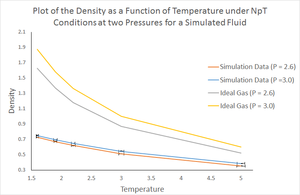
). The results are plotted in figure 11.

Firstly, it can be said that there is significant difference between the results at $P=2.6$ and $P=3.0$ since there the standard error bars do not overlap. The results presented can be explained by consideration of the ideal gas equation, rearranged to make the number density the subject (below).

$\frac{\mathrm{N}}{V}=\frac{P}{k_B\mathrm{T}}$

The results show that with increasing temperature at constant pressure, the density is decreased. This is as expected since density is inversely proportional to the temperature (as seen from the equation above). This also makes sense conceptually since with increased temperature, the particles have greater kinetic energy hence will move around more and 'occupy more space' on average. This means the particles will be more separated per unit volume at higher temperatures, corresponding to a lower density.

For a given temperature, an increase in pressure leads to an increase in density. This is again explainable by the direct relationship between density and pressure. Conceptually, by applying a greater pressure to a given volume, the particles are force closer together on average hence the system has a greater density.

It is clear that the densities calculated from the ideal gas equation are much higher than those calculated by simulation. In an ideal gas, it is assumed that there are no interactions, attractive or repulsive, other than elastic collisions. Without these pairwise repulsive interactions, ion average, the particles can be found at much smaller inter-atomic separations hence the bulk system will have a higher density. In the simulation, the Lennard-Jones potential is applied meaning at small separations, there is repulsion between the particles, as seen from the rapid increase in $\varphi (r)$ on the left-hand side of the Lennard-Jones potential plot. The particles cannot approach each other as closely, relative to when assuming ideal gas behaviour, hence the densities are lower.

Lastly, it is found that the discrepancy between the density at $P=2.6$ and $P=3.0$ is larger when assuming ideal gas behaviour than for the simulation results. This is likely because the ideal gas equation neglects forces of attraction and repulsion. For an ideal gas, the density is just proportional to the pressure at constant temperature, however the simulation is more representative of a physical system and likely uses equations with terms that consider these forces. This means density and pressure have a more complicated relationship than that given by the ideal gas equation.

Thermostats and Barostats

Though we have chosen to fix the temperature to a constant value in the NpT calculations, the actual temperature, $\mathrm{T}$, in fact fluctuates around the inputted/desired temperature, $\mathfrak{𝔗}$. To compensate for this difference and ensure the temperature does not significantly deviate from the desired temperature over the course of the simulation, the velocity at every timestep is multiplied by a constant, $\gamma$. This scaling factor ensures that $\mathrm{T}=\mathfrak{𝔗}$ after each timestep. The following details how $\gamma$ is derived.

$E_K=\frac{3}{2}N{k}_B\mathrm{T}$

$\frac{1}{2}\sum _i{m}_i{v_i}^2=\frac{3}{2}N{k}_B\mathrm{T}$

$\frac{1}{2}\sum _i{m}_i(\gamma v_i{)}^2=\frac{3}{2}N{k}_B\mathfrak{𝔗}$

By summing the second and third equations:

$\frac{1}{2}\sum _i{m}_i{v_i}^2+\frac{1}{2}\sum _i{m}_i(\gamma v_i{)}^2=\frac{3}{2}N{k}_B\mathrm{T}+\frac{3}{2}N{k}_B\mathfrak{𝔗}$

Since $\gamma$ is a constant, it can be taken outside the summation:

$\sum _i{m}_i{v_i}^2+{\gamma }^2\sum _i{m}_i{v_i}^2=3N{k}_B(\mathrm{T}+\mathfrak{𝔗})$

$\left(\sum _i{m}_i{v_i}^2\right)({\gamma }^2+1)=3N{k}_B(\mathrm{T}+\mathfrak{𝔗})$

Substituting in the second equation:

$(3N{k}_B\mathrm{T})({\gamma }^2+1)=3N{k}_B(\mathrm{T}+\mathfrak{𝔗})$

${\gamma }^2+1=\frac{\mathrm{T}+\mathfrak{𝔗}}{\mathrm{T}}$

${\gamma }^2=\frac{\mathrm{T}+\mathfrak{𝔗}}{\mathrm{T}}-1$

${\gamma }^2=\frac{\mathrm{T}+\mathfrak{𝔗}}{\mathrm{T}}-\frac{\mathrm{T}}{\mathrm{T}}$

${\gamma }^2=\frac{\mathfrak{𝔗}}{\mathrm{T}}$

$$\begin{gathered} \therefore \\ \gamma =\sqrt{\frac{\mathfrak{𝔗}}{\mathrm{T}}} \end{gathered}$$

Examining the input scripts

Within the input script for each simulation, the following lines of code are present:

fix aves all ave/time 100 1000 100000 v_dens v_temp v_press v_dens2 v_temp2 v_press2
run 100000

fix aves is used to calculate averages for variables used as 'arguments' in the command. Once again, all applies this command to all atom types. In words, the av/time 100 1000 100000 part says "output the global time-averaged values using every 100th timestep and do this 1000 times in order to calculate the average for every 100000 timesteps". Since we run for just 100000 timesteps (run 100000), we only get one average outputted per variable from this command. Since our timestep was set to t = 0.0025, we simulate 250 time units.

The variables we want averages for are named 'dens', 'temp', 'press', 'dens2', 'temp2' and 'press2'. The v_* notation is similar to the ${*} notation, but is more suitable to recalling a variable with a value that changes during the simulation.

Calculating heat capacities using statistical physics

Figure 12: Heat capacity per volume vs. temperature graph for a simulated fluid at two densities

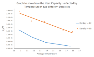
Much like in the previous section, 10 simulations were run (2 sets of 5 temperatures), however they were instead run under NVT conditions (constant number of atoms, volume and temperature). Under these conditions, 2 densities were defined (

$\rho =0.2$

and

$\rho =0.8$

) and temperatures between

$\mathrm{T}=2.0$

and

$\mathrm{T}=2.8$

were used. The fluctuations in total energy of the system under isothermal conditions can be used to calculate the heat capacity,

$C_V$

using the equation below.

$C_V=\frac{\partial \mathrm{E}}{\partial \mathrm{T}}={\mathrm{N}}^2\frac{⟨{\mathrm{E}}^2⟩-⟨\mathrm{E}{⟩}^2}{k_B{\mathrm{T}}^2}$

The results

The heat capacities per volume, $\frac{C_V}{V}$, for all 10 simulations was obtained and the results can be seen in figure 12. The heat capacity has been divided by the volume to allow for comparison between the two densities used. At $\rho =0.2$, the volume is calculated to equal 16875 units, while at $\rho =0.8$ the volume is 4218.75 units, i.e. a quadrupling of the density has resulting in a quarter of the volume since the number of atoms is constant.

The results show that at both densities, an increase in temperature results in a decrease in heat capacity. This result is not what is expected from theory. Heat capacity is defined as the amount of heat required to increase the temperature of a substance by one degree. We therefore expect the heat capacity to increase with temperature because at high temperature, it takes more heat energy to raise the temperature another degree, relative to at low temperatures. The results obtained here contradict this understanding.

According to the results, at an given temperature, the heat capacity is higher at the higher density. At higher density, atoms are on average closer together. It may be expected that when providing heat energy, this heat can be conducted better in a more dense medium since the atoms are closer together hence it should be easier to raise the temperature of the substance. The results again contradict this argument.

The input script

The following is an example an the input script used with conditions of $\rho =0.2$ and $\mathrm{T}=2.0$.

### SECTION 1: DEFINE SIMULATION BOX GEOMETRY ###
lattice sc 0.2
region box block 0 15 0 15 0 15
create_box 1 box
create_atoms 1 box

### S2: DEFINE PHYSICAL PROPERTIES OF ATOMS ###
mass 1 1.0
pair_style lj/cut/opt 3.0
pair_coeff 1 1 1.0 1.0
neighbor 2.0 bin

### S3: SPECIFY THE REQUIRED THERMODYNAMIC STATE ###
variable T equal 2.0
variable timestep equal 0.0025

### S4: ASSIGN ATOMIC VELOCITIES ###
velocity all create ${T} 12345 dist gaussian rot yes mom yes

### S5: SPECIFY ENSEMBLE ###
timestep ${timestep}
fix nve all nve

### S6: THERMODYNAMIC OUTPUT CONTROL ###
thermo_style custom time etotal temp press
thermo 10

### S7: RECORD TRAJECTORY ###
dump traj all custom 1000 output-1 id x y z

### S8: RUN SIMULATION TO MELT CRYSTAL ###
run 10000
unfix nve
reset_timestep 0

### S9: BRING SYSTEM TO REQUIRED STATE ###
variable tdamp equal ${timestep}*100
fix nvt all nvt temp ${T} ${T} ${tdamp}
run 10000
reset_timestep 0

### S10: MEASURE SYSTEM STATE ###
thermo_style custom step etotal temp vol atoms
variable etotal equal etotal
variable etotal2 equal etotal*etotal
variable temp equal temp
variable temp2 equal temp*temp
fix aves all ave/time 100 1000 100000 v_temp v_etotal v_etotal2
unfix nvt
fix nve all nve
run 100000

### S11: DEFINE USEFUL VARIABLES ###
variable avetemp equal f_aves[1]
variable aveetotal equal f_aves[2]
variable varetotal equal (f_aves[3]-f_aves[2]*f_aves[2])
variable volume equal vol
variable N equal atoms
variable N2 equal atoms*atoms

### S12: CALCULATE HEAT CAPACITY ###
variable heatcap equal ((${N2}*${varetotal})/(${avetemp}*${avetemp}))
variable cvV equal (${heatcap}/${volume})

### S13: PRINT DESIRED VALUES ###
print "Averages"
print "--------"
print "Temperature: ${avetemp}"
print "ETotal: ${aveetotal}"
print "Volume: ${volume}"
print "HeatCapacity: ${heatcap}"
print "Cv/V: ${cvV}"

Structural properties and the radial distribution function

Figure 13: RDF vs. distance plots

Figure 14: Running integral for the RDF plot of an FCC lattice solid with call-outs at the plateaus

Figure 15: Illustration of a cross-section of an FCC lattice, containing 4 unit cells

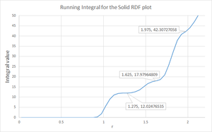
The radial distribution function (RDF), $g(r)$, is useful in determining the how the number density varies with distance from a given particle. The RDF for a model solid, liquid and gas were plotted (figure 13). The solid requires an FCC lattice to be defined (reference for phase diagram of a Lennard-Jones system). The conditions are given below:

Solid: $\rho =1.2$, $\mathrm{T}=1.2$,
Liquid: $\rho =0.8$, $\mathrm{T}=1.2$,
Gas: $\rho =0.05$, $\mathrm{T}=1.2$.

It can be seen from figure 13, there are more peaks for the solid and fewer for the liquid and just a smooth curve for the gas. The more peaks in the RDF plot, the greater the long range ordering of the system. This result is therefore as expected since a solid, with a fix regular structure, is more ordered than a gas which is not ordered due to weak interactions between particles. In the case of the solid, the RDF can be used to calculate the coordination number of a particle. The first peak corresponds to interactions with the closest neighbours, the second with the second closest and so on. By conducting a running integral for the RDF and evaluating the integral value corresponding to $r$ values for these peaks, the coordination number can be evaluated.

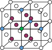
From reading off the integral values at the plateaus in figure 14, the coordination number can be determined. For the first peak, there are 12 closest neighbours. For the second peak, there are 6 (18-12) second closest neighbours. Finally, for the third peak, there are 24 (42-18) third closest neighbours. Therefore, the coordination number for the model FCC solid begins with 2, 6, 24. Figure 15 attempts to illustrate the first two coordination numbers. Focusing on the green atom, there are 12 purple neighbours (8 of which are shown). These are the closest neighbours since they are found $\frac{\sqrt{2}}{2}$ unit cell lengths away from the green atom. There are 6 blue atoms (5 of which are shown) 1 unit cell side length away, hence these are the second closest neighbours.

The lattice spacing is calculated as follows:

The number density, $\rho =\frac{N}{V}$ is given as 1.2. Since there are 4 lattice points per unit cell of an FFC lattice, $N=4$ hence $V=\frac{10}{3}$. Since the unit cell is a cube, cube rooting gives the length of a unit cell side: $$\begin{gathered} V=\sqrt[3]{\frac{10}{3}}=1.49380 \\ (5d.p.) \end{gathered}$$.

Dynamical properties and the diffusion coefficient

Mean Squared Displacement

The diffusion coefficient, $D$, can be calculated from first determining the mean squared displacement (MSD) of a system and utilising the following equation.

$D=\frac{1}{6}\frac{\partial ⟨r^2(t)⟩}{\partial t}$

The mean squared displacement in this case relates to how 'far' on average a particle moves within the system while on a random path.

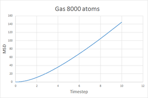
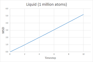
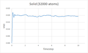
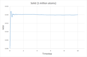
The MSD at each timestep was calculated for simulations of a gas, liquid and solid and plotted against the timestep and the results are shown below.

	8000 (g, l) / 32000 (s) atom simulation (Run on HPC)	~ 1 million atom simulation (Provided)
Gas MSD vs. timestep graph
Gas diffusion coefficient	2.54E+00	2.54E+00
Liquid MSD vs. timestep graph
Liquid diffusion coefficient	8.49E-02	8.73E-02
Solid (FCC) MSD vs. timestep graph
Solid diffusion coefficient	1.04E-05	6.79E-06

As expected, the diffusion coefficient is largest for a gas, then liquid and finally smallest for a solid. Since the gaseous state is the least dense of the three, it is easily to imagine that a gas particle would travel further and more freely than a liquid and much more than a solid, hence the MSD for a gas should be the largest. A solid is highly constrained to a specific structure meaning the particles cannot move very freely and so a smaller MSD is expected. The plots show the MSD for a gas reaches over 140 units, compared to 5 units for a liquid and just 0.02 units for a solid.

For the gas MSD vs. time graph, some curative can be seen between 0 and 2 time units. This is because, initially, the particles are not moving randomly, but rather in a relatively straight line at a relatively constant velocity until collisions begins. 'The distance travel is proportional to time and so the MSD is proportional to the time squared' (Reference), hence giving curvature to the line at the start. After collisions, the velocities are much more random giving rise to a straighter line.

In contrast to the gas and liquid curves, the graph for the solid shows the MSD rapidly increases and plateaus. This probably relates to the solid quickly 'snapping' from the starting lattice to a structure with reduced pairwise repulsions. The system then equilibrates to this specific structure with minor movement of the particles after this.

Going from gas to liquid to solid, the discrepancy between $D$ between the 8000 and 1 million atom simulations increases, however they are still acceptably similar. With more atoms simulated, the results of the simulation better represent a physical system hence the coefficient obtained from the 1 million atoms simulation is probably more accurate.

Velocity Autocorrelation Function

The normalised velocity autocorrelation function for a 1D harmonic oscillator

The velocity autocorrelation function, $C(\tau )$ relates the current velocity of a particle to its previous velocity in the simulation. This function is useful as an alternative method for determining the diffusion coefficient.

$C(\tau )=\frac{\underset{-\mathrm{\infty }}{\overset{\mathrm{\infty }}{\int }}v(t)v(t+\tau )\mathrm{d}t}{\underset{-\mathrm{\infty }}{\overset{\mathrm{\infty }}{\int }}{v}^2(t)\mathrm{d}t}$

The velocity is the first derivative of position with respect to time:

$v(t)=\frac{\mathrm{d}x(t)}{\mathrm{d}t}$

Substituting in the equation for position for the harmonic oscillator:

$v(t)=\frac{\mathrm{d}(Acos(\omega t+\varphi ))}{\mathrm{d}t}$

$$\begin{gathered} v(t)=-Aw \\ sin(\omega t+\varphi ) \end{gathered}$$

$$\begin{gathered} v(t+\tau )=-A\omega \\ sin(\omega (t+\tau )+\varphi ) \end{gathered}$$

Substituting these into the first equation:

$$\begin{gathered} C(\tau )=\frac{\underset{-\mathrm{\infty }}{\overset{\mathrm{\infty }}{\int }}(-A\omega \\ sin(\omega t+\varphi ))\cdot (-A\omega \\ sin(\omega (t+\tau )+\varphi )\mathrm{d}t}{\underset{-\mathrm{\infty }}{\overset{\mathrm{\infty }}{\int }}(A^2{\omega }^2 \\ si{n}^2(\omega t+\varphi ))\mathrm{d}t} \end{gathered}$$

$C(\tau )=\frac{\underset{-\mathrm{\infty }}{\overset{\mathrm{\infty }}{\int }}(sin(\omega t+\varphi ))\cdot (sin(\omega (t+\tau )+\varphi )\mathrm{d}t}{\underset{-\mathrm{\infty }}{\overset{\mathrm{\infty }}{\int }}si{n}^2(\omega t+\varphi )\mathrm{d}t}$

Applying a standard trigonometric identity to separate the $\tau$ term in the sine function:

$C(\tau )=\frac{\underset{-\mathrm{\infty }}{\overset{\mathrm{\infty }}{\int }}(sin(\omega t+\varphi ))[sin(\omega t+\varphi )cos(\omega \tau )+cos(\omega t+\varphi )sin(\omega \tau )]\mathrm{d}t}{\underset{-\mathrm{\infty }}{\overset{\mathrm{\infty }}{\int }}si{n}^2(\omega t+\varphi )\mathrm{d}t}$

Since $\omega \tau$ is a constant in this integration:

$C(\tau )=\frac{cos(\omega \tau )\underset{-\mathrm{\infty }}{\overset{\mathrm{\infty }}{\int }}si{n}^2(\omega t+\varphi )\mathrm{d}t+sin(\omega \tau )\underset{-\mathrm{\infty }}{\overset{\mathrm{\infty }}{\int }}sin(\omega t+\varphi )cos(\omega t+\varphi )\mathrm{d}t}{\underset{-\mathrm{\infty }}{\overset{\mathrm{\infty }}{\int }}si{n}^2(\omega t+\varphi )\mathrm{d}t}$

$C(\tau )=cos(\omega \tau )+\frac{sin(\omega \tau )\underset{-\mathrm{\infty }}{\overset{\mathrm{\infty }}{\int }}sin(\omega t+\varphi )cos(\omega t+\varphi )\mathrm{d}t}{\underset{-\mathrm{\infty }}{\overset{\mathrm{\infty }}{\int }}si{n}^2(\omega t+\varphi )\mathrm{d}t}$

Since sine is an antisymmetric function and cosine is a symmetric function, $sin(\omega t+\varphi )cos(\omega t+\varphi )$ is an antisymmetric function. The integral of an antisymmetric function between ±$\mathrm{\infty }$ is zero, therefore the equation cancels down to:

$C(\tau )=cos(\omega \tau )$

VACFs for liquid and solid simulations

Figure 16: VACFs for liquid and solid simulations and the harmonic oscillator

Figure 16, right, is a plot the VACF as a function of timestep between 0 and 500. For the liquid and solid, $C(\tau )$ is seen to decrease to a negative value, reaching a minimum and then equilibrating to zero after some time. At time zero, $C(\tau )$ is at a maximum since the velocity at this time is exactly equal to its previous velocity (i.e. the velocity at time zero). As the simulation is run, interactions between particles causes the velocity to change hence gradually becoming less like the previous velocity. $C(\tau )$ becomes negative and reaches a minimum when there is a collision that causes a change in direction of a particle. Collisions result in random motion and trajectories hence the 'memory' of previous velocities is 'lost' and so the correlation tends to zero at infinite time. Since velocity is a vector, it has a direction, hence giving a negative value for $C(\tau )$. The minimum is more negative for the solid because the particles are closer packed than in a liquid hence are more likely to collide and change direction with greater force.

In contrast, $C(\tau )$ for the harmonic oscillator, where $\omega =\frac{1}{2\pi }$ is plotted as the green line and is seen to oscillate between ± 1 without equilbrating to zero. In the stretching phase of the harmonic oscillator, the potential energy increases and so the kinetic energy (hence velocity) of the particle decreases eventually reaching zero at the maximum stretch distance. This corresponds to the upwards sloping part of the cosine function, e.g. between approximately 110 and 230 timesteps. When relaxing back to the original position, the direction of velocity becomes negative, increasing in magnitude initially and then slowing to zero again at the minimum stretch distance. This corresponds to the downwards sloping sections, e.g. between 0 and approx. 110 timesteps. Since the harmonic oscillator does not stop, just changes direction, $C(\tau )$ does not tend to zero because there is no random motion just predictable oscillation between positive and negative directions of velocity.

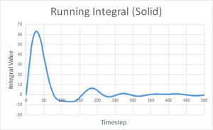
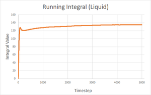
Calculating D from VACFs

$D=\frac{1}{3}\underset{0}{\overset{\mathrm{\infty }}{\int }}C(\tau )\mathrm{d}\tau$

	Solid	Liquid	Gas
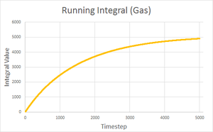
Running Integral plot	Solid	Liquid	Gas
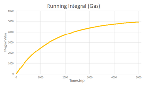Final integral after 5000 timesteps	-0.276	146.833	4941.881
Calculated diffusion coefficient	D = 0.0921	D = 48.9	D = 1647

Calculating D from VACFs for 1 million atoms

	Solid	Liquid	Gas
Running Integral plot	Solid, 1 million atoms	Liquid, 1 million atoms	Gas, 1 million atoms
Final integral after 5000 timesteps	0.0683	135.137	4902.699
Calculated diffusion coefficient	D = 0.0228	D = 45.0	D = 1634

Discussion of results

For both sets of simulations (1 million atoms and otherwise), the same general trend is observed; the gas has the highest diffusion coefficient and the solid the smallest. This trend is in agreement with that found for the MSD calculations and also theory. However, the diffusion coefficients calculated from VACFs are all greater in magnitude than those from the MSD. This may be due to the approximation applied to calculate the integral values of the VACFs. The trapezium rule was used which provides an approximate value for the actual integral for the plot. Having said this, it is unclear whether the error associated with the trapezium rule at every point is significant enough to account for, for example, the difference of 2 orders of magnitude between the gas diffusion coefficient for 1 million atoms.