
Rep:AD5215LS
Overall feedback: the tasks were completed well and conveyed a good level of understanding. The scientific report was well written and had an interesting motivation. However, it greater attention could have been placed on where certain information should go: for example, background theory is usually in the introduction. Some explanations would have benefited from a more precise use of scientific language and concepts. The motivation of molecular gastronomy was never related to the specific results/conclusions. The conclusion was a bit sparse. Overall good level of knowledge and understanding was conveyed.
Tasks
Section 2: Introduction
TASK: Open the file HO.xls. In it, the velocity-Verlet algorithm is used to model the behaviour of a classical harmonic oscillator. Complete the three columns "ANALYTICAL", "ERROR", and "ENERGY": "ANALYTICAL" should contain the value of the classical solution for the position at time , "ERROR" should contain the absolute difference between "ANALYTICAL" and the velocity-Verlet solution (i.e. ERROR should always be positive -- make sure you leave the half step rows blank!), and "ENERGY" should contain the total energy of the oscillator for the velocity-Verlet solution. Remember that the position of a classical harmonic oscillator is given by (the values of , , and are worked out for you in the sheet).
Excel file attached here.
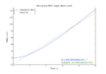
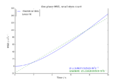
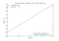
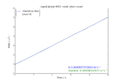
TASK: For the default timestep value, 0.1, estimate the positions of the maxima in the ERROR column as a function of time. Make a plot showing these values as a function of time, and fit an appropriate function to the data.

TASK: Experiment with different values of the timestep. What sort of a timestep do you need to use to ensure that the total energy does not change by more than 1% over the course of your "simulation"? Why do you think it is important to monitor the total energy of a physical system when modelling its behaviour numerically?
The change in energy goes down as the timestep value becomes smaller. For a timestep of 0.25 the change in energy is 1.58% while for a timestep of 0.05 the change in energy is 0.06% . The energy change is 1.01% for a timestep of 0.2 . A timestep that is too large could lead to the simulation effectively "missing" any changes in the system that happen on a shorter timescale than that of the timestep. Therefore, it is important to monitor the energy to ensure that the change is not too drastic and we are observing the behaviour of the system closely.
TASK: For a single Lennard-Jones interaction, , find the separation, , at which the potential energy is zero. What is the force at this separation? Find the equilibrium separation, , and work out the well depth (). Evaluate the integrals , , and when .
Find the separation at which the potential energy is zero

FInd the force at
The force is the derivative of potential wrt to distance:

At separation this will be
.JPG)
Equilibrium separation and well depth<\span>
The equilibrium separation is the separation when

The well depth at this separation is

negative epsilon
Integrals


TASK: Estimate the number of water molecules in 1ml of water under standard conditions. Estimate the volume of water molecules under standard conditions.
N molecules occupy 1 mL. Therefore, the volume of 1 molecule of water will be
The volume of 1000 molecules will be
TASK: Consider an atom at position in a cubic simulation box which runs from to . In a single timestep, it moves along the vector . At what point does it end up, after the periodic boundary conditions have been applied?
It ends up at position (0.2, 0.1, 0.7).
TASK: The Lennard-Jones parameters for argon are . If the LJ cutoff is , what is it in real units? What is the well depth in ? What is the reduced temperature in real units?
for 1 particle
For a mole of particles:
Section 3: Equilibration
TASK: Why do you think giving atoms random starting coordinates causes problems in simulations? Hint: what happens if two atoms happen to be generated close together?
Randomly generated positions can lead to two atoms being very close together, which would result in a large repulsive potential. This would then affect any propagation in time of the system, which would lead to undesirable behaviour, especially when using larger timesteps. The system would most likely behave "appropriately" for small enough timesteps, but this would require running longer simulations. This would be less effective; a larger timestep that still results in an accurate simulation is ideal. good!
TASK: Satisfy yourself that this lattice spacing corresponds to a number density of lattice points of . Consider instead a face-centred cubic lattice with a lattice point number density of 1.2. What is the side length of the cubic unit cell?
Density: ---> Length:
For a simple cubic lattice with , the length, l, is:
For a face-centered cubic lattice with , the length, l, is:
TASK: Consider again the face-centred cubic lattice from the previous task. How many atoms would be created by the create_atoms command if you had defined that lattice instead?
The box would still contain lattice units. For an FCC there are 4 atoms per lattice unit. Therefore the total number of atoms would be atoms.
TASK: Using the LAMMPS manual, find the purpose of the following commands in the input script:
mass 1 1.0
pair_style lj/cut 3.0
pair_coeff * * 1.0 1.0
"Mass" sets the mass of a particular type of atom (in this case, the mass of type 1 atoms is 1). "Pair" refers to pair potentials. The lj/cut command computes the 12/6 Lennard-Jones potential, cut sets the cut-off for r. Pair_coeff sets the values for the 2 parameters, sigma and epsilon.
TASK: Given that we are specifying and , which integration algorithm are we going to use?
Velocity Verlet. A simple Verlet algorithm wouldn't require the initial velocity, but would instead require .
TASK: Look at the lines below.
### SPECIFY TIMESTEP ###
variable timestep equal 0.001
variable n_steps equal floor(100/${timestep})
timestep ${timestep}

### RUN SIMULATION ###
run ${n_steps}
run 100000
The second line (starting "variable timestep...") tells LAMMPS that if it encounters the text ${timestep} on a subsequent line, it should replace it by the value given. In this case, the value ${timestep} is always replaced by 0.001. In light of this, what do you think the purpose of these lines is? Why not just write:
timestep 0.001
run 100000
The line "variable timestep equal 0.001" defines a variable timestep which is the assigned a value. This allows for the variable to be called later on if needed. This is convenient for the user as it means that if the same variable is required multiple times (in this case, the variable timestep is called twice) changing its value is easier, as this only needs to be done once (in the line defining the variable).
Section 4: Running simulations under specific conditions
TASK: We need to choose so that the temperature is correct if we multiply every velocity . We can write two equations:
Solve these to determine .

TASK: Use the manual page to find out the importance of the three numbers 100 1000 100000. How often will values of the temperature, etc., be sampled for the average? How many measurements contribute to the average? Looking to the following line, how much time will you simulate?
From the manual, the structure of the command is "ave/time Nevery Nrepeat Nfreq".
- Nevery (100) = use input values every this many timesteps (total no. of data points is 100,000 so this will give 1000 values to be averaged in the next step; records an average of 100 values)
- Nrepeat (1000) = no. of times to use input values for calculating averages (i.e. average over 1000 values)
- Nfreq (100,000) = calculate averages every this many timesteps (same no. specified in the "run" command)
The timestep is 0.0025 and the simulation runs for 100,000 steps. Therefore we are simulating a total time of 250 seconds .
Section 7: Dynamical properties and the diffusion coefficient
TASK: In the theoretical section at the beginning, the equation for the evolution of the position of a 1D harmonic oscillator as a function of time was given. Using this, evaluate the normalised velocity autocorrelation function for a 1D harmonic oscillator (it is analytic!):
For a HO model:

The VACF is given by

We evaluate the two integrals separately. Integral 2 is

Using .JPG) we can write
we can write

Integral 1 is

Using ![]() we can write
we can write

We evaluate the last integral separately.

Substituting this back we obtain:

Substituting I1 and I2 into the formula for C we obtain

Sin is an odd function, i.e.  . Thus

There is definitely a shorter way of doing this, but yes.
Report
Abstract
Solid, liquid and gaseous systems were modeled using LAMMPS and a 12-6 Lennard-Jones forcefield. A suitable timestep of 0.0025 was determined. Simulations were run to obtain thermodynamic data (temperatures, pressures, densities, heat capacities). Calculated densities were found to be lower than those predicted by the ideal gas law. The simulated heat capacities showed a trend, decreasing with increasing temperature. The RDF was calculated for systems in all three phases. As expected, the RDF for a solid showed peaks decaying in amplitude. Lattice spacings and coordination numbers for the solid FCC lattice were calculated. The MSD and the VACF were plotted for the same three systems and the diffusion coefficient was calculated for both measurements. The two methods did not result in identical values; still, the difference was only 0.67% for the diffusion coefficients in the gas phase. Good, concise abstract that summaries main results. Perhaps 1 sentence of motivation would have been nice.
Introduction
Food constitutes a huge part of our lives, whether we actively think about it or not. Cooking, in some form or other, has been around ever since the first human realised that fire makes raw meat tastier and more convenient to eat. Nowadays, the food industry is enormous and cooking has become a successful blend of art and science. Perhaps the most pertinent example of this is molecular gastronomy, a subdiscipline of food science that seeks to investigate the physical and chemical transformations of ingredients during the cooking process. In their review, Balham et al refer to molecular gastronomy as an "emerging scientific discipline".[1]
In fact, molecular gastronomy relies heavily on processes such as gelification and infusion and on materials such as gels, foams and powders. It also uses equipment that is heavily reminiscent of a laboratory - some kitchens are fitted with butane burners, syringes and dehydrators.
Clever presentations and unusual sensations and are piquing the interest of many people; in some places, molecular gastronomy restaurants have become tourist attractions.[2] Simulating the thermodynamic properties of systems can provide a better understanding of physical systems and can lead to the growth and development of this industry.
An interesting topic and motivation! An explicit connection between gastronomy and the results you intend to present/discuss would be nice. For example how is the diffusion coefficient relevant? The introduction of a scientific paper usually includes the background theory, such as in your case, the equations for diffusion coefficient. You have included this in the methodology, which while logical, is not standard practice for most papers/journals.
Aims and Objectives
- become familiar with LAMMPS and how simulating a physical system works
- model the behaviour of systems under the 12-6 Lennard-Jones potential
- calculate the physical properties (temperature, pressure, density, etc) of a system using such simulations
- comparing the results of the simulations to theory (e.g. simulated density vs density given by the ideal gas law)
- calculating the diffusion coefficient for systems in different phases (gas, liquid, solid) by two different methods (from the MSD and from the VACF)
Methods
General methods
A 12-6 Lennard-Jones system was modeled usings LAMMPS and all simulations were run using Imperial's High Performance Computer. The potential for such a system is given by[3]:
All calculations used reduced units:, and The Lennard-Jones parameters and were set to 1.0 for all simulations. The cutoff for Lennard-Jones interactions was set at r*=3 unless otherwise stated. The mass of the atoms was set to 1.0. The temperature, pressure, lattice density and timestep values were varied. For all calculations the velocity Verlet algorithm was employed. The atoms were assigned random velocities within the simulation, while ensuring that the Boltzmann distribution of states is followed.
Determining a suitable timestep
A simple cubic lattice with a density of 0.8 was defined and the simulation was populated with 1000 atoms (10 x 10 x 10 dimensions). The ensemble was defined as the microcanonical (NVE) ensemble. Five values for the timestep were tested: 0.015, 0.01, 0.0075, 0.0025, 0.001 and each simulation was run for a total time of 100 seconds. Values for the energy, temperature and pressure of the system were recorded at each step.
Variation of density with temperature and pressure
A simple cubic lattice with a density of 0.8 was defined and the simulation was populated with 3375 atoms (15 x 15 x 15 dimensions). The timestep for all simulations was set to 0.0025. The ensemble was defined as NPT and 10 different thermodynamic states were simulated (two pressures, 2.5 and 3.5, each associated with five temperatures: 3.0, 6.0, 9.0, 12.0 and 15.0). Values for the energy, temperature and pressure of the system were recorded at each step, as well as average values for the density, temperature and pressure of the system at the end of the simulation. Plots of density vs time were obtained, both for the simulated data and for densities predicted by the ideal gas law[3],
Heat capacity calculations
A simple cubic lattice with a density of 0.2 was defined and populated with 3375 atoms. The timestep for all simulations was set to 0.0025. An NVT ensemble was simulated for five temperatures: 2.0, 2.2, 2.4, 2.6 and 2.8. Then, a subsequent simulation was run to establish an NVE ensemble and measure the properties of the system. Average values for temperature, energy, volume and heat capacity were calculated. This procedure was repeated for a simple cubic lattice with a density of 0.8. An example input script can be found here.
The heat capacity of a system is given by[3]:
where E is the internal energy and
is the variance in internal energy. The term is required because LAMMPS automatically outputs the energy per atom, not the total energy.

RDF calculations
Three systems (a liquid, a solid and a gas) were modeled and populated with 3375 atoms each. Temperature and density values were taken from the Lennard-Jones fluid phase diagram[4] reproduced in Fig. 1. These were defined as:
- solid: fcc lattice, temperature 1.2, density 1.2;
- liquid: sc lattice, temperature 1.2 , density 0.8;
- vapour: sc lattice, temperature 1.2, density 0.05.
The ensemble was defined as NVT. The timestep for all simulations was set to 0.002. The trajectories of the atoms were recorded and VMD was used to calculate the radial distribution function and its integral from these trajectories. The data was then analysed using Python.
Diffusion coefficient calculations
The same three systems as above were modeled, this time with 8000 atoms each. The timestep was set to 0.002 and each simulation was run for 5000 steps. The Lennard-Jones cutoff was set to 3.2. The ensemble was defined as NVT. The mean squared displacement (MSD) and the velocity autocorrelation function (VACF) at each step were calculated for all systems. The data was analysed using Python. The MSD plots were fitted to a straight line and the gradient was used to calculate the diffusion coefficient. The VACF integrals were plotted as a function of time and, again, used to calculate the diffusion coefficient. The same data analysis was conducted using supplied data which modeled larger systems.
The MSD is a measure of the deviation of the position of a particle with respect to a reference position over time. It can be thought of as a measure of how much the system moves over time. The MSD is given by:
The diffusion coefficient (D) can be calculated from the MSD, using[5]:
The VACF is given by
and is effectively a measure of how closely related the velocity of a particle is (at time t) to its initial velocity (at time t=0). This correlation is "perturbed" by collisions; at very long times (i.e. when t tends to infinity) we expect the VACF to be zero, as all particles will have collided at least once and their velocities will be uncorrelated.
The diffusion coefficient is proportional to the integral of the VACF[5]:
Good, I could reproduce your results with this information.
Results & Discussion
Equilibration
Plots of energy, temperature and pressure vs time were obtained for a timestep value of 0.001. These are reproduced in Fig. 2-4. It can be seen that all three plots reach a "plateau" very quickly; equilibration is almost instantaneous. The values oscillate slightly, as a result of the approximations required by the simulation. These oscillations are however very small (note the scale of the y-axis).
 |
 |
 |
An important feature of these simulations is the timestep. The shorter the timestep the more "accurate" the simulation, but the more computational power this will require. In this case, plots of the total energy vs time were obtained for all five timestep values (Fig. 5).

The lowest energy is given by timestep values of 0.001 and 0.0025. These energies are almost identical; the 0.001 energy is lower, but the difference in energies is only 0.005%. In addition to this, for simulating a total time of e.g. 100s, ts = 0.0025 requires 40,000 steps, while ts = 0.001 requires 100,000 steps. Therefore, the 0.0025 timestep is the better choice, as the difference in energies is not large enough to warrant the use of more computational power (as required by the 0.001 timestep). The 0.015 timestep is a poor choice. Not only is the energy the highest of the five, but, unlike in the other four cases, the system does not reach equilibrium and the energy keeps increasing.
Based on this data, further simulations were run using a 0.0025 timestep (unless a different value was required by the lab script).
Equilibration is not typically discussed in the results section of a scientific paper. Simply "systems were equilibrium for X timesteps/unit with a timestep of Y" would be sufficient. You get the marks for the task however.
Densities and the ideal gas law
Plots of density vs temperature for two different pressures are reproduced in Fig. 6. The density given by the ideal gas law was also calculated and plotted on the same graph.

It can be seen that the results of the simulation do not match those given by the theoretical approach. This is because the ideal gas law does not take into account any interaction between particles, i.e. it assumes that the gas behaves ideally. In the Lennard-Jones model the particles experience attractive and repulsive forces; the repulsive forces dominate be careful to convey precise meaning: when do repulsive forces dominate? and cause the system to be more diffuse and thus have a lower simulated density.
The discrepancy between theory and simulation increases with increasing pressure because this "pushes" the particles closer together and increases the effect of Lennard-Jones forces. It also increases with decreasing temperature; at low temperatures, the Lennard-Jones forces dominate, while at high temperatures thermal motion is more significant. I understand what you are trying to say here, however a more precise/succinct explanation would have been helpful. For example, rationalising your results in terms of the potential energy surface and available thermal energy ... "at the high temperature limit, LJ particles have enough kinetic energy to easily surmount all kinetic energy barriers in the PES", or something more elegantly worded.
Heat capacities
The variation in heat capacity with temperature is shown in Fig. 7. The system is under the NVE ensemble so we are dealing with the isochoric heat capacity, CV.

The heat capacity decreases with increasing temperature. This agrees with the formula for heat capacity, which shows inverse proportionality to temperature. However, this is not the full extent of the explanation.
Heat capacity is a measure of how much energy (heat) is required to increase the temperature of a system. At higher temperatures more energetic states become available and the spacing between them decreases - this makes populating higher states easier, leading to a decrease in heat capacity.
In addition to this, increasing the temperature can lead to a phase change and thus to an increase in the degrees of freedom available to the system (e.g. melting causes a solid - rigid, fewer degrees of freedom - to change into a liquid).
The Radial Distribution Function (RDF)

The radial distribution function for a solid, liquid and gas is reproduced in Fig. 8. The RDF shows how a system is arranged, relative to the position of one particle in the system; effectively, it is a measure of long-range order. A peak corresponds to a shell of atoms around the central particle. The intensity of the peak (effectively its integral) is proportional to the number of atoms within this shell.
All three RDFs (vapour, liquid, solid) show an initial peak, but differ in their behaviour at longer distances. The RDF for a system in the gas phase rapidly reaches a value of 1 and plateaus. This is because a gas is, by its very nature, disordered. Atoms are free to move and they tend to disperse, not arrange themselves in shells. The RDF for a liquid oscillates slightly after the initial peak but also plateaus at 1 after a short distance. The initial peak corresponds to a solvation shell around the central particle. The subsequent smaller peaks show that a liquid has some degree of order - the forces between the particles are strong enough to restrict their movement to a degree.

The RDF for the solid system is different to the other two, as it shows long-range order. It does not plateau but instead shows peaks of decreasing intensity. This can be explained by looking at the structure of the solid crystal. This was defined in the simulation as a face-centred cubic (FCC) lattice, shown in Figure 9. The particles are arranged in shells, at distances which depend on the lattice spacing of the crystal. This can be calculated from the lattice density (1.2).
The first three peaks in the RDF plot correspond to the first three neighbouring sites of the central particle, coloured in blue, purple and green respectively. The lattice spacing and the coordination number of each site can be calculated by considering the geometry of the crystal:
- Shell 1 is found at and holds atoms.
- Shell 2 is found at and holds atoms.
- Shell 3 is found at and holds atoms.
These values agree with those found by the RDF. The coordination numbers match those calculated from the running integral, which has values of 12.15, 17.98 and 42.3 respectively.
The diffusion coefficient, D
Plots of the total mean squared displacement vs time are reproduced in Appendix A. Plots of the VACF vs time are reproduced in Appendix B. Plots of the VACF running integral vs time are reproduced in Appendix B.
Figure 10 below shows the time evolution of the VACF for a solid, a liquid and a gas, as well as for an ideal harmonic oscillator.

The VACF is effectively a measure of how closely related the velocity of a particle is (at time t) to its initial velocity (at time t=0). This correlation is "perturbed" by collisions or by interactions with other particles; at very long times (i.e. when t tends to infinity) we expect the VACF to be zero and the velocities to be uncorrelated. What does the first minimum indicate?
The harmonic oscillator shows perfectly oscillatory behaviour, with constant amplitude in time: the velocity goes from an initial state to an uncorrelated one and then back to the initial state. The solid shows similar behaviour: the VACF oscillates about 0 but dampens with time. This is because in a solid the atoms have fixed positions in a lattice; the forces between the particles are strong and these will oscillate in place for a while. The VACF takes much longer to reach zero than in the case of a liquid or a gas. The gas VACF tends slowly to zero; the interactions between particles in a gas are minimal, which means that the velocity at time is not very different from an initial velocity. A liquid is somewhere in-between these two phases: the particles have more freedom of movement than they do in a solid, but the attractive forces are strong enough to cause a perturbation in the velocities; the VACF shows a very slight oscillation, but then quickly dampens to zero.
The diffusion coefficients can be calculated in two different ways, either from the gradient of an MSD plot or from the integral of the VACF. These calculations were performed and the D values are given in Table 1.
| Phase | MSD data | VACF data | ||
|---|---|---|---|---|
| Small simulation | Large simulation | Small simulation | Large simulation | |
| Gas | 2.536 | 2.542 | 3.294 | 3.268 |
| Gas, linear region | 3.317 | 3.217 | --- | --- |
| Liquid | 0.085 | 0.087 | 0.098 | 0.090 |
| Solid | 5.825 x 10⁻⁷ | 4.391 x 10⁻⁴ | -1.845 x 10^-4 | 4.558 x 10^-5 |
The largest error in the case of the MSD measurements comes from the fact that the gas phase gives rise to a curved plot, which cannot be feasibly fitted to a straight line. This is because particles in a gas will diffuse readily and thus the system will take longer to reach equilibrium (the linear region) than, say, a liquid. A longer simulation that would allow the system to reach equilibrium and then collect a larger amount of data would provide a more accurate result, as in this case the linear region that was used only comprised about 20% of the total data. In the case of a liquid, the MSD function is linear and provides the best fit and thus the most accurate result. The MSD for a solid establishes linear behaviour quickly, as the particles are "fixed". The diffusion coefficient values are very small; this shows that in a solid no diffusion (or almost none) takes place.
In the case of the VACF measurements the largest error comes from using the trapezium rule to compute the integral. The smaller the timestep, the more accurate the measurement - in this case the timestep is relatively small but some error still remains.
The errors in both of these measurements cause the diffusion coefficients to differ slightly. The difference between the MSD- and VACF-calculated diffusion coefficients are 0.67%, 15.3% and 31780% for the gas, liquid and solid phases respectively. The difference in the case of the solid phase is incredibly large but not significant as we have established diffusion is not a significant process for solids. The difference for the liquid phase is quite small and likely comes from the poor fit of the MSD plot and the short duration of the simulation.
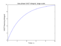
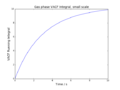
Appendix A: MSD plots
-
 Gas phase MSD (large scale)
 -
 Gas phase MSD, linear region (large scale)
 -
 Gas phase MSD (small scale)
 -
 Gas phase MSD, linear region (small scale)
 -
 Liquid phase MSD (large scale)
 -
 Liquid phase MSD (small scale
 -
 Solid phase MSD (large scale)
 -
 Solid phase MSD (small scale)


Appendix B: VACF running integral plots
-
 Gas phase (large scale)
 -
 Gas phase (small scale)
 -
 Liquid phase (large scale)
 -
 Liquid phase (small scale)
 -
 Solid phase (large scale)
 -
 Solid phase (small scale)


Conclusion
This lab provided insight into the thermodynamic properties of systems and how these change with phase, temperature, pressure. Of course, the systems investigated were small, but modeling larger, more complicated systems is possible and could prove useful. A particular domain where this kind of research would be invaluable is, as previously mentioned, molecular gastronomy: understanding phase changes and the properties of liquids, solids and gels can lead to the advancement of this (pseudo)-scientific discipline.
This conclusion is a bit short: it should include a summary of the results, and perhaps a short outlook. It would also be nice to convey the importance/meaning of your results and conclusions in the context of molecular gastronomy, which you motivated your study with, but have not mentioned since the introduction.
- ↑ P. Barham, L. H. Skibsted, W. L. P. Bredie and J. Risbo, Symp. A Q. J. Mod. Foreign Lit., 2010, 2313–2365.
- ↑ D. Tüzünkan and A. Albayrak, Procedia - Soc. Behav. Sci., 2015, 195, 446–452.
- ↑ 3.0 3.1 3.2 P. Atkins, J. De Paula, Physical Chemistry, OUP Oxford, 9th edn., 2009.
- ↑ J. P. Hansen and L. Verlet, Phys. Rev., 1969, 184, 151–161.
- ↑ 5.0 5.1 O. J. Eder, J. Chem. Phys., 1977, 66, 3866–3870.