Rep:AC5116 Ising Monte

Introduction

Variously sized 2D Ising Model Lattices were simulated in the canonical ensemble (NVT) with Monte Carlo simulation to find the average energies, $⟨E⟩$, and magnetisations, $⟨M⟩$. These simulations were carried out for a range of temperatures to show the temperature dependence of these properties. A fairly sharp drop in magnetisation corresponding to a phase transition was observed. The critical point of this phase transition (the Curie temperature, $T_C$) was found for each of the lattices by finding the temperature at which the heat capacity of the system peaks at. Utilising a scaling formula, $T_{C,L}=A/L+T_{C\mathrm{\infty }}$, and plotting $T_{C,L}$(Curie temperature of a finite lattice of side size L) vs. $1/L$(1/length of side) it was found that the Curie temperature at infinite temperature, $T_{C,\mathrm{\infty }}$ , was (2.30 ± 0.02) K. This shows a fairly good correspondence to the analytical solution of $T_{C,\mathrm{\infty }}$ ≈ 2.269 K.

Note. In this lab the interaction, $J=k_B$ and given we shall be working reduced units (divide by $k_B$) in the code,$J=1.0$, in reduced units.

The Ising model represents the system as a discrete lattice of spins (1D or higher dimensions) which may adopt a spin of either $+1$ or $-1$. The interaction between 2 neighbouring spins is given by $-J{s}_i{s}_j$, where $s_i$ is the spin at lattice site i and j is a nearest neighbour of i. The total energy of the system is given by:

$$\begin{gathered} -\frac{1}{2}J\sum _i^N\sum _{j \\ \in \\ \mathrm{n}\mathrm{e}\mathrm{i}\mathrm{g}\mathrm{h}\mathrm{b}\mathrm{o}\mathrm{u}\mathrm{r}\mathrm{s}\left(i\right)}{s}_i{s}_j</mathThismodel,unlikemeanfieldtheory,allowsforfluctuationsi{n}^{\prime }concentratio{n}^{\prime }ofspins.Thismakesitusefulfornotonlymodellingferromagnetic(andantiferromagneticsystems),butasawayofaccountingforinteractionsbetween2liquids(whereupanddownspinsrepresenttwodifferentsubstances).The2DIsinglatticeisespeciallyimportant,asitisaverysimplesystemthatexhibitsaphasetransition.Belowthecriticaltemperatureofthisphasetransition,theCurietemperature,thesystemhasspontaneousmagnetisation(when<math>J>0 \end{gathered}$$), and hence has a net magnetisation equal in magnitude to the number of particles and above it has $⟨M⟩=0$ (no net magnetisation). This phase transition can be understood by the favourable interactions of between spins of the same sign in an ordered phase dominating the free energy below the Curie temperature, however, above this temperature, the entropic term of the free energy dominates and disordered configurations of the system become more likely, such that $⟨M⟩=0$.

Monte Carlo Simulation is a useful technique for simulating a 2D Ising Lattice in the canonical ensemble because it allows for average properties to be built by only incorporating configurations of the lattice that matter significantly, has a high Boltzmann factor that is, at a specified temperature into the averages. This technique is called importance sampling. As the canonical ensemble will be used to simulate this system, the temperature is simply a parameter that controls the distribution of states.

Section 1: Introduction to the Ising Model

TASK: Show that the lowest possible energy for the Ising model is$E=-DNJ$, where $D$ is the number of dimensions and $N$ is the total number of spins. What is the multiplicity of this state? Calculate its entropy.

Lowest energy configuration for all spins the same (for $J$> 0, ferromagnetic). i.e. $s_i=s_j\mathrm{\forall }i,j$

Because $s_i$may take on the value only the values ± 1, no matter if all spins are +1 or -1 gives the same minimum energy. Hence the total energy is:

$$\begin{gathered} E_{\mathrm{m}\mathrm{i}\mathrm{n}}=-\frac{1}{2}J\sum _i^N\sum _{j \\ \in \mathrm{n}\mathrm{e}\mathrm{i}\mathrm{g}\mathrm{h}\mathrm{b}\mathrm{o}\mathrm{u}\mathrm{r}\mathrm{s}\left(i\right)}{s}_i{s}_j=-\frac{1}{2}J\sum _i^N\sum _{j \\ \in \mathrm{n}\mathrm{e}\mathrm{i}\mathrm{g}\mathrm{h}\mathrm{b}\mathrm{o}\mathrm{u}\mathrm{r}\mathrm{s}\left(i\right)}1 \end{gathered}$$

For a given number of dimensions,$D$, the number of immediate neighbours to a given spin is given by $2D$, as there is another spin either 'side' of the particle in each dimension. Hence the second sum simple reduces to $2D$:

$E_{\mathrm{m}\mathrm{i}\mathrm{n}}=-\frac{1}{2}J\sum _i^{N}2D=$

$=-\frac{1}{2}J\left(2ND\right)$

Hence:

$E_{\mathrm{m}\mathrm{i}\mathrm{n}}=-DNJ$

As there are 2 possible configurations for which the system has this energy (all spin up or all spin down) the multiplicity of the system is 2, $\mathrm{\Omega }=2$. Hence, using the Boltzmann Entropy Formula:

$S=k_B\ln 2$

TASK: Imagine that the system is in the lowest energy configuration. To move to a different state, one of the spins must spontaneously change direction ("flip"). What is the change in energy if this happens ()? How much entropy does the system gain by doing so?

Changing one spin’s sign changes, the interactions with its $2D$ neighbours to become repulsive instead of attractive and go from –$J$ to +$J$. As the sign is flipped 2D attractive interactions are lost and 2D repulsive interactions are gained. Hence the energy of the system with a single spin flipped is: $E=-DNJ+2DJ-(-2DJ)=-DJ(N+4)$. Hence for $D=3$, the energy increase is:$\mathrm{\Delta }E=+4DJ=+12J$

Entropy change can be calculated by, where $\mathrm{\Omega }$ is the multiplicity :

$\mathrm{\Delta }S=k_B(\ln {\mathrm{\Omega }}_f-\ln {\mathrm{\Omega }}_i)=k_B\ln \frac{{\mathrm{\Omega }}_f}{{\mathrm{\Omega }}_i}$

For the initial configuration (all up or all down) ${\mathrm{\Omega }}_i=2$ and with one spin flipped the multiplicity is ${\mathrm{\Omega }}_f=2000$ (any one of the 1000 spins flipped in either of the 2 starting states).

Hence:

$\mathrm{\Delta }S=k_B\ln 1000$

TASK: Calculate the magnetisation of the 1D and 2D lattices in figure 1. What magnetisation would you expect to observe for an Ising lattice with at absolute zero?

1D Lattice: 3 x $\uparrow$, 2 x $\downarrow$. Hence, $M=3*1+2*(-1)=+1$

• 2D Lattice: 13 x $\uparrow$, 12 x $\uparrow$. Hence, $M=13*1+12*(-1)=+1$

• 3D lattice with at , all spins point either up or down (adopting one of the lowest energy configurations), hence: $M=\pm 1000$

Section 2: Calculating the energy and magnetisation

TASK: complete the functions energy() and magnetisation(), which should return the energy of the lattice and the total magnetisation, respectively. In the energy() function you may assume that $J=1.0$ at all times (in fact, we are working in reduced units in which $J=k_B$, but there will be more information about this in later sections). Do not worry about the efficiency of the code at the moment — we will address the speed in a later part of the experiment.

An instance of the Ising Lattice class, il, has a variable called 'lattice' which is a 2D array (of dimensions specified in on initialising the instance) containing a random arrangement of +1 and -1, representing the up and down spins of a 2D Ising Lattice.

The code below computes the energy by iterating over every single spin in the lattice array and calculates the interaction with its adjacent neighbours to the left and below, and only in these directions to prevent double counting. n-1 / m-1 is used to specify the neighbour as in Python when the index of a list goes below 0, it loops around and counts from the last member of the list. However, if the index is increased over the size of the lattice, it raises an indexing error. Alternatively self.lattice[m][n-1] can be replaced with self.lattice[m][(n+1)%self.n_cols], and similarly for the other direction, which gives the interactions of the nearest neighbours to the right and above the spin at m, n. %self.n_cols applies modulus to index so it doesn't go over the number of columns.

The magnetisation code is simpler; it just iterates over both the rows and columns and sums the values of each spin.

   def energy(self):
       "Return the total energy of the current lattice configuration."
       J=1
       energy = 0.0
       for m,row in enumerate(self.lattice):
           for n,sigma in enumerate(self.lattice):
               energy-=J*(self.lattice[m][n]*self.lattice[m][(n-1)]+self.lattice[m][n]*self.lattice[m-1][n])
       return energy
   
   def magnetisation(self):
       "Return the total magnetisation of the current lattice configuration."
       magnetisation = 0
       for i in self.lattice:
           for j in i:
               magnetisation += j
       return magnetisation

TASK: Run the ILcheck.py script from the IPython Qt console using the command

%run ILcheck.py

The displayed window has a series of control buttons in the bottom left, one of which will allow you to export the figure as a PNG image. Save an image of the ILcheck.py output, and include it in your report.

Running the ILcheck.py script confirms this method of calculating the energy and magnetisation indeed yields the correct results, as seen in the figure below.

Figure X:Output of the ILcheck.py script. Demonstrates the energy and magnetisation code working correctly.

Section 3: Introduction To Monte Carlo Simulation

Chat stuff about how Monte Carlo Works

TASK: How many configurations are available to a system with 100 spins? To evaluate these expressions, we have to calculate the energy and magnetisation for each of these configurations, then perform the sum. Let's be very, very, generous, and say that we can analyse $1\times 10^9$ configurations per second with our computer. How long will it take to evaluate a single value of ${⟨M⟩}_T$?

As each site in an Ising Lattice has 2 possible states (spin up/spin down) there is $2^N$ possible configurations of spins($N$ being the total number of spins). For a system of 100 spins, there is $2^{100}\approx 1.268\times 10^{30}$ potential configurations. If a computer could analyse these configurations at $1\times 10^9\mathrm{c}\mathrm{o}\mathrm{n}\mathrm{f}\mathrm{i}\mathrm{g}\mathrm{u}\mathrm{r}\mathrm{a}\mathrm{t}\mathrm{i}\mathrm{o}\mathrm{n}\mathrm{s}{\mathrm{s}}^{\mathrm{-}\mathrm{1}}$, it would take $1.268\times 10^{21}\mathrm{s}$, which is roughly $40,200,000,000,000$ years, longer than the age of the universe!

Hence. as it is not possible to exactly calculate the partition function of a moderately sized Ising lattice, we need to sample only the configurations that contribute most significantly to the distribution of states, the Boltzmann distribution, as for many configurations $\exp (-\frac{E(\alpha )}{k_{B}T})$ is very small. This is called Importance Sampling and is achieved by the Metropolis Monte Carlo method.

TASK: Implement a single cycle of the above algorithm in the montecarlocycle(T) function. This function should return the energy of your lattice and the magnetisation at the end of the cycle. You may assume that the energy returned by your energy() function is in units of $k_B$! Complete the statistics() function. This should return the following quantities whenever it is called: $<E>,<E^2>,<M>,<M^2>$, and the number of Monte Carlo steps that have elapsed.

In this implementation of the Metropolis Monte Carlo method, the energy of an initial configuration ($E_0$) is calculated, then the configuration is altered slightly by flipping a random spin. If the energy of the new configuration ($E_1$) is lower than the previous one, it is kept and the algorithm moves on to the next Monte Carlo step. This is because if a configuration of lower energy will have a larger $\exp (-\frac{E(\alpha )}{k_{B}T})$ and hence contribute to more to the distribution than the previous. If upon flipping a spin the energy of the system increases, the probability of transition ($\exp (-\frac{\mathrm{\Delta }E}{k_{B}T})$, where $\mathrm{\Delta }E=E_1-E_0$ ) is compared to a random number between 0 and 1. If the $\exp (-\frac{\mathrm{\Delta }E}{k_{B}T})$ is greater than or equal to the random number, the new configuration and energy is accepted. This ensures that very few extremely high energy configurations that contribute little to the distribution are sampled. In this simulation, the energies of accepted configurations from each Monte Carlo step are summed up to be used to calculate the average energy of the system.

The code used to incorporate the Monte Carlo algorithm into the Ising Lattice class is shown below:

def montecarlostep(self, T):
    # complete this function so that it performs a single Monte Carlo step
    #stores the energy and magnetisation of the lattice.
    en0 = self.energy()
    mn0 = self.magnetisation()
    #chooses a random spin to flip
    random_i = np.random.choice(range(0, self.n_rows))
    random_j = np.random.choice(range(0, self.n_cols))
    #the following line will choose a random number in the rang e[0,1) for you
    random_number = np.random.random()
    #flips a spin
    self.lattice[random_i][random_j]=-1*self.lattice[random_i][random_j]
    #stores the new energy and calculates the change
    en1 = self.energy()
    deltaE = en1-en0
    #if deltaE is +ve, checks exp(-deltaE/T) vs. a random number
    if deltaE >0:
        if random_number > np.exp(-deltaE / T):
            #Rejects config if probability is too low compared to random number - flips spin back
            self.lattice[random_i][random_j]=-self.lattice[random_i][random_j] 
    else:
        #New configuration accepted; en0 and mn0 is redefined to be that of the new config.
        en0 = en1
        mn0 = self.magnetisation()
    #increases the number of cycles by one 
    self.n_cycles += 1
    #adds to the energy, energy squared, magnetisation and magnetisation squared variables, used to calculate averages when statistics() is called.    
    self.E += en0; self.E2 += en0**2; self.M += mn0; self.M2 += mn0**2
    
    return en0, mn0

When the above method is called it first flips a random spin, and then checks whether the new configuration meets the rejection criteria (carried out first as there is only one scenario in which a configuration may be rejected, but two in which it can be accepted), and if not the new configuration is accepted. If the perturbed configuration is not rejected, en0 and mn0 are updated. en0 and mn0 are used to add to self.E, self.E2, self.M and self.M2, which at this point are just sums of the observables returned by a Monte Carlo step and are converted into averages when the statistics() method is called.

def statistics(self):

   # complete this function so that it calculates the correct values for the averages of E, E*E (E2), M, M*M (M2), and returns them
   #E,E2,M and M2 values have all been added up in monte carlo step, simply divided by the number of cycles to give the averages of these values.
   self.E = self.E/self.n_cycles
   self.E2 = self.E2/self.n_cycles
   self.M = self.M/self.n_cycles
   self.M2 = self.M2/self.n_cycles
   return self.E , self.E2, self.M, self.M2, self.n_cycles

TASK: If $T<T_C$, do you expect a spontaneous magnetisation (i.e. do you expect $⟨M⟩\ne 0$)? When the state of the simulation appears to stop changing (when you have reached an equilibrium state), use the controls to export the output to PNG and attach this to your report. You should also include the output from your statistics() function.

Testing the Monte Carlo simulation by running ILanim.py shows how the system's configuration, energy and magnetisation varies with the number of Monte Carlo steps and approaches equilibrium(once energy and magnetisation have reached a constant value). The energy/magnetisation vs. Monte Carlo step plots below show the approach of an 8x8 system at 1 K to equilibrium. The outputted average energy and magnetisation, along with the average of the corresponding squares, were (in with energies in units of $k_B$ per spin): $E$ = -1.548 , $E^2$= 2.677, $M$ = 0.738, $M^2$ = 0.648. These averaged properties are significantly different from the final equilibrium values (from the figure below, $E$ = -2 and $M$ = 1). This is because the averages are currently taken over all of the Monte Carlo cycles, opposed to only averaging over steps after the simulation has equilibrated (where $E$ and $M$ fluctuate about a single value); this will be corrected later.

The output of ILanim.py for an 8x8 system at 1 K.

It is expected that below $T_C$, the system should have spontaneous magnetisation, with an energy and magnetisation fluctuating about $E$=-2 and $M$= ±1 (per spin) respectively, which changes steeply over the Curie temperature. This suggests that 1 K is below the Curie temperature for an 8x8 system.

Section 4: Accelerating the code

The code, as it is currently, is very slow. In order to speed it this up, the code for calculating the energy and magnetisation needs to be improved. Instead of using a double for loop to calculate both magnetisation and energy, numpy functions will be used instead.

In order to see how much faster the changes make the code, the script ILtimetrial.py is run. This script runs 2000 Monte Carlo steps of a 25 x 25 Ising lattice at 1 K and outputs the elapsed time. This was repeated 8 times and the results are shown in the table below:

TASK: Use the script ILtimetrial.py to record how long your current version of IsingLattice.py takes to perform 2000 Monte Carlo steps. This will vary, depending on what else the computer happens to be doing, so perform repeats and report the error in your average!

t1/s	t2/s	t3/s	t4/s	t5/s	t6/s	t7/s	t8/s	< t >/s	σt/s
5.884258	5.782945	5.715886	5.870607	5.769787	6.087371	5.902848	5.835443	5.856143125	0.105808334

The average time that was taken for this example simulation to run on the old code was $⟨\tau ⟩=5.86\mathrm{s}$, with a standard deviation of $0.11\mathrm{s}$

TASK: Look at the documentation for the NumPy sum function. You should be able to modify your magnetisation() function so that it uses this to evaluate M. The energy is a little trickier. Familiarise yourself with the NumPy roll and multiply functions, and use these to replace your energy double loop (you will need to call roll and multiply twice!).

The numpy.roll (np.roll) function shifts all the elements of an array by a given over a specified number of steps, and elements that would be shifted off the array are re-introduced in the first index. Describing this visually with matrices:

$\left[\begin{array}{ccc}{s}_{11}& s_{12}& s_{13}\\ s_{21}& s_{22}& s_{23}\\ s_{31}& s_{32}& s_{33}\end{array}\right]\underset{}{\overset{\text{np.roll(self.lattice,1,1)}}{\to }}\left[\begin{array}{ccc}{s}_{13}& s_{11}& s_{12}\\ s_{23}& s_{21}& s_{22}\\ s_{33}& s_{31}& s_{32}\end{array}\right]$

Here np.roll(self.lattice,1,1) shifts the elements of the matrix along to the next row. np.multiply can then be used to multiply the shifted matrix by the original, element-wise, such that in the resulting matrix has elements $S_{ij}=s_{ij}{s}_{ij-1}$. Hence each of these elements is the interaction of the spin $s_{ij}$ with its neighbour in the left direction(with periodic boundaries). Using the function np.sum, summing every element of the array up, on this product matrix hence gives the contribution to the total interaction energy of particles with the particle to left. This is then repeated, using np.roll(self.lattice,1,0) which instead shifts elements in the spin array down a row, to give the contribution to the total energy due to interactions between particles immediately below a given particle. These are summed to give the total energy of the system(no factor of a half needed as interactions in only 2 directions are calculated, so aren't double counted). The code for all this comes out to be:

def energy(self):
    energy=-np.sum(np.multiply(self.lattice,np.roll(self.lattice,1,1)))
    energy-=np.sum(np.multiply(self.lattice,np.roll(self.lattice,1,0)))
    return energy
   

The np.sum function mentioned before is also useful for calculating the magnetisation of the system. As the magnetisation is simply the sum of every element in the self.lattice array, the faster code for magnetisation is simply:

def magnetisation(self):
    return np.sum(self.lattice)

TASK: Use the script ILtimetrial.py to record how long your new version of IsingLattice.py takes to perform 2000 Monte Carlo steps. This will vary, depending on what else the computer happens to be doing, so perform repeats and report the error in your average!

Utilising these functions drastically increased the speed of performing the 2000 Monte Carlo steps, by almost a factor of 20! The new average run time was found to be:$⟨\tau ⟩=\mathrm{0}\mathrm{.}\mathrm{3}\mathrm{3}\mathrm{1}\mathrm{s}$ with a standard deviation of $0.0169\mathrm{s}$. The raw data for the ILtimetrial.py runs are shown in the table below. Although the "old" code for calculating energy did essentially the same thing as the "new" code, the new code prevents the need for a double for loop every time energy or magnetisation is calculated. Considering for a 25 by 25 lattice there are 625 spins to loop over and energy is calculated twice in each Monte Carlo step (and magnetisation once), even though the process of iterating once may be relatively fast, over a large number of steps this adds a lot of computational time. For the 25x25 system in ILtimetrial.py the system must calculate the energy/magnetisation at 3,750,000 lattice sites in total over the course of the realtively short simulation.

t1/s	t2/s	t3/s	t4/s	t5/s	t6/s	t7/s	t8/s	tav/s	σt/s
0.352151	0.314524	0.349517	0.332359	0.321895	0.316048	0.313276	0.348684	0.331057	0.016890

Section 5: The Effect of Temperature - Part 1 Correcting Averaging Code

As the code currently is, the averages calculated don't correctly correspond with the average values of the equilibrium distribution. In order to rectify this issue, we want to start taking averages only once the system has reached equilibrium, with a constant average energy and magnetisation. To know when to start taking averages, some experimentation with a variety of system sizes and temperatures needs to be carried out, to determine the effect of these properties on the number of cycles before equilibration. The table below summarises some of these investigations.

TASK: The script ILfinalframe.py runs for a given number of cycles at a given temperature, then plots a depiction of the final lattice state as well as graphs of the energy and magnetisation as a function of cycle number. This is much quicker than animating every frame! Experiment with different temperature and lattice sizes. How many cycles are typically needed for the system to go from its random starting position to the equilibrium state? Modify your statistics() and montecarlostep() functions so that the first N cycles of the simulation are ignored when calculating the averages. You should state in your report what period you chose to ignore, and include graphs from ILfinalframe.py to illustrate your motivation in choosing this figure.

$T$/K	Lattice Size	Approx No. of Steps to Equilibration	Magnitude of Energy Fluctuations	Image
0.25 K	2 x 2	<10	N/A
	4 x 4	≈113	N/A
	8 x 8	≈500-1000	N/A
	16 x 16	≈ 8000	N/A
	32 x 32	≈ 140,000	N/A
1 K	2 x 2	<10	± 1
	4 x 4	≈70	±0.5
	8 x 8	≈500	N/A
	16 x 16	≈10000	N/A
	32 x 32	≈ 80,000	N/A
2.5 K	2 x 2	<10
	4 x 4	Very fast < 200	0.5
	8 x 8	<1000	N/A
	16 x 16	<1000	≈0.25
	32 x 32	<8000	Tiny. Fluctuations in M much larger.

A few general trends can be seen from this relatively small collection of data. Firstly, larger lattice sizes, in general, take longer to reach equilibrium. This makes sense as there are far more possible configurations to sample (the total number of possible configurations follows $2^N$), so sampling configuration space takes longer. Also, flipping a single spin has a much smaller effect on energy, so more configurations are likely to be accepted that increase the energy and the takes the system away from equilibrium. Another trend that can be seen is that at higher temperatures, the systems tend to reach equilibrium much faster, albeit with significantly greater fluctuations. The magnitude of these 'temperature' fluctuations appears to decrease with increasing lattice size; flipping a single spin in a larger lattice has a much smaller effect on the net magnetisation + energy, so the magnitude of fluctuations(per spin) are smaller. In the table above the plots for T = 2.5 K should be above the Curie temperature for most of the systems, as can be seen graphically by the disorder in the final frame lattices.

Comparison of the number of cycles after which averages are taken and the number of cycles taken for the system to reach equilibrium (at 0.25 K) vs. lattice size. The cutoff is larger than the actual equilibrium number of steps, as to minimise the risk of starting averaging too early.

For the code to run efficiently, the cutoff (after which averaging starts) must be a function of system size, otherwise, it will take small systems as long for the code to run as larger systems, despite reaching equilibrium much quicker than larger systems. Although formally the number of configurations the system can adopt should follow $2^N$, where$N$ is the number of spins, many of these $2^N$ configurations are too high in energy to be visited during a Monte Carlo system and equilibrium would be reached much faster than this number of steps (the point of sampling in the first place). Hence instead of scaling the equilibrium cutoff exponentially the number of particles, it was made to scale with the square of the length of the lattice, $L$, and hence proportional to $N$. The parameters of this quadratic were chosen such that they overestimated the time for equilibration, compared to the data in the table above, but the cut off was of a similar order of magnitude (as to prevent starting averaging prior to actually reaching equilibration, in case the test cases above were remarkably fast). This quadratic scaling with $L$ should work well for lattice sizes between 2 and 32 (which are investigated later in this report), but may not hold up for significantly larger lattices.

To define the cutoff, a new property of the IsingLattice class was defined, self.n_cutoff. The value of this is determined on initialising an instance of the class and was related to $L$ by the expression:

$n_{cutoff}=200L^2+1000$

The corresponding code in the __init__ method being:

   def __init__(self, n_rows, n_cols):
       self.n_cutoff = 200*self.n_rows*self.n_cols+1000

The comparison of this cutoff compared to the number of steps till equilibrium at 0.25 K for several lattice sizes in the figure above. This cutoff is implemented into the code by modifying the montecarlostep() and statistics() methods as follows:

   def montecarlostep(self, T):
       # complete this function so that it performs a single Monte Carlo step
       #stores the energy and magnetisation of the lattice.
       en0 = self.energy()
       mn0 = self.magnetisation()
       #chooses a random spin to flip
       random_i = np.random.choice(range(0, self.n_rows))
       random_j = np.random.choice(range(0, self.n_cols))
       #the following line will choose a random number in the rang e[0,1) for you
       random_number = np.random.random()
       #flips a spin
       self.lattice[random_i][random_j]=-1*self.lattice[random_i][random_j]
       #stores the new energy and calculates the change
       en1 = self.energy()
       deltaE = en1-en0
       #print(deltaE)
       if deltaE >0:
           if random_number > np.exp(-deltaE / T):
           #Rejects config if probability is too low compared to random number - flips spin back
              self.lattice[random_i][random_j]=-self.lattice[random_i][random_j] 
           
       else:
           #New configuration accepted; en0 and mn0 is redefined to be that of the new config.
           en0 = en1
           mn0 = self.magnetisation()
       self.n_cycles += 1
       #only if the number of cycles is greater than the cutoff(see __init__ method) will the E, E2, M and M2 start to be calculated
       if self.n_cycles > self.n_cutoff:
           self.E += en0; self.E2 += en0**2; self.M += mn0; self.M2 += mn0**2
       return en0, mn0

   def statistics(self):
       # complete this function so that it calculates the correct values for the averages of E, E*E (E2), M, M*M (M2), and returns them
       #E,E2,M and M2 values have all been added up in monte carlo step, simply divided by the number of cycles to give the averages of these values.
       self.n_cycles = self.n_cycles - self.n_cutoff
       print(self.n_cycles)
       self.E = self.E/self.n_cycles
       self.E2 = self.E2/self.n_cycles
       self.M = self.M/self.n_cycles
       self.M2 = self.M2/self.n_cycles
       return self.E , self.E2, self.M, self.M2, self.n_cycles

An if statement has simply been added to the end of the Monte-Carlo cycle that checks whether the cycle number is currently greater than the 'cutoff' or not, and if so $E,E^2,M,M^2$ are added to the totals for these properties. When the statistics function is called, it simply divides these totals by the number of Monte-Carlo cycles elapsed, minus the number of cycles before the cutoff. As the system should be equilibrated before this cutoff, the average is now corrected.

Section 5: The Effect of Temperature - Part 2 Temperature Curves

TASK: Use ILtemperaturerange.py to plot the average energy and magnetisation for each temperature, with error bars, for an $8\times 8$ lattice. Use your intuition and results from the script ILfinalframe.py to estimate how many cycles each simulation should be. The temperature range of 0.25 to 5.0 is sufficient. Use as many temperature points as you feel necessary to illustrate the trend, but do not use a temperature spacing larger than 0.5. The NumPy function savetxt() stores your array of output data on disk — you will need it later. Save the file as 8x8.dat so that you know which lattice size it came from.

The temperature range calculations (for the 8x8 lattice, and all future runs of different lattice sizes) were run between $T=0.25-5\mathrm{K}$ with a step size $0.05\mathrm{K}$. The number of monte carlo cycles used was different for each lattice size, as the larger lattices had later cutoffs. To make the number of cycles used in averaging the same for every system, the runtime of $n_{cutoff}(L)+50,000$ was used, such that the average quantities were calculated from 50,000 Monte-Carlo steps.

The average energy vs. T and magnetisation vs. T curves produced by Monte-Carlo simulation of an 8x8 Ising Lattice. The error bars, that are plotted for every 5 data points, are calculated from the standard deviation of the plotted average, calculated from $\sqrt{⟨X^2⟩-⟨X{⟩}^2}$. Standard error was not plotted as the error bars would be too small to be visible.

The resulting average magnetisation and average energy vs. temperature curves are shown in the figures below. The energy-temperature curve shows an initially flat line at the minimum possible energy of the system, which starts to increase steeply around 2 K, then slowly starts to plateau beyond 2.5 K, with an energy close to 0.

The magnetisation-temperature curve has a similar behaviour, $⟨M⟩$ starts as a flat line with the maximum magnetisation of the system ($⟨M⟩\pm 1$ per spin) and then abruptly drops. However, instead of plateauing like the energy graph, the average magnetisation instead oscillates about $⟨M⟩=0$, with a decaying amplitude. The abrupt changes in properties of the system are indicative of a phase change of the system, between the highly ordered state with $⟨M⟩=1$ to the much more disordered state that has $⟨M⟩=0$. The temperature of this transition ($T_c$) can't be as well read from these plots as with the exact 2D solution of the infinite lattice, where there is a discontinuity between the $⟨M⟩=1$ and $⟨M⟩=0$ phases at $T=T_c$.

The error bars in these plots increase with temperature. This is to be expected as there are more 'thermal' fluctuations for higher temperatures than lower; more configurations with different energies contribute more significantly to the average energy (and hence a larger standard deviation arises).

Section 6: The Effect of Lattice Size

TASK: Repeat the final task of the previous section for the following lattice sizes: 2x2, 4x4, 8x8, 16x16, 32x32. Make sure that you name each datafile that your produce after the corresponding lattice size! Write a Python script to make a plot showing the energy per spin versus temperature for each of your lattice sizes. Hint: the NumPy loadtxt function is the reverse of the savetxt function, and can be used to read your previously saved files into the script. Repeat this for the magnetisation. As before, use the plot controls to save your a PNG image of your plot and attach this to the report. How big a lattice do you think is big enough to capture the long range fluctuations?

The ILtemperaturerange.py script was run again for more lattice sizes; 2x2, 4x4, 16x16 and 32x32. The runtimes of each Monte Carlo simulation, for each temperature, as given by the expression in the previous section, were 51800, 54200, 102200, 255800, for 2x2, 4x4, 16x16 and 32x32 respectively. The resulting plots are shown in the next two figures.

Figure: Average energy/ magnetisation vs. Temperature for 2x2, 4x4, 8x8, 16x16 and 32x32 Ising Lattices, shown on the same plot. Error bars have been excluded here for clarity.

All 5 systems (including 8x8) all exhibit very similar behaviours with temperature. Apart from the smaller systems (2x2, 4x4) the Energy-Temperature Curves nearly completely overlap with each other and approach similar average energies per spin. The smaller systems (especially 2x2) don't reach the same energy per spin, due to the smaller number of spins in the system resulting and fewer possible configurations restricting the maximum possible entropy of the system and maximum possible energy (there isn't enough possible disorder to balance out a positive energy). In the 2x2 system there are 8 possible configurations (Media:AC5116 2 by 2 configs.jpg) 2 of which are degenerate with the lowest possible energy,$E$ = -2J per spin , 4 with a medium energy, $E$ = 0, and 2 with $E$ = +2$J$ per spin. This cumbersome distribution of energies gives a much lower potential maximum average energy, as entropy can't compensate for the occupation of the E=+2$J$ states until very high temperatures.

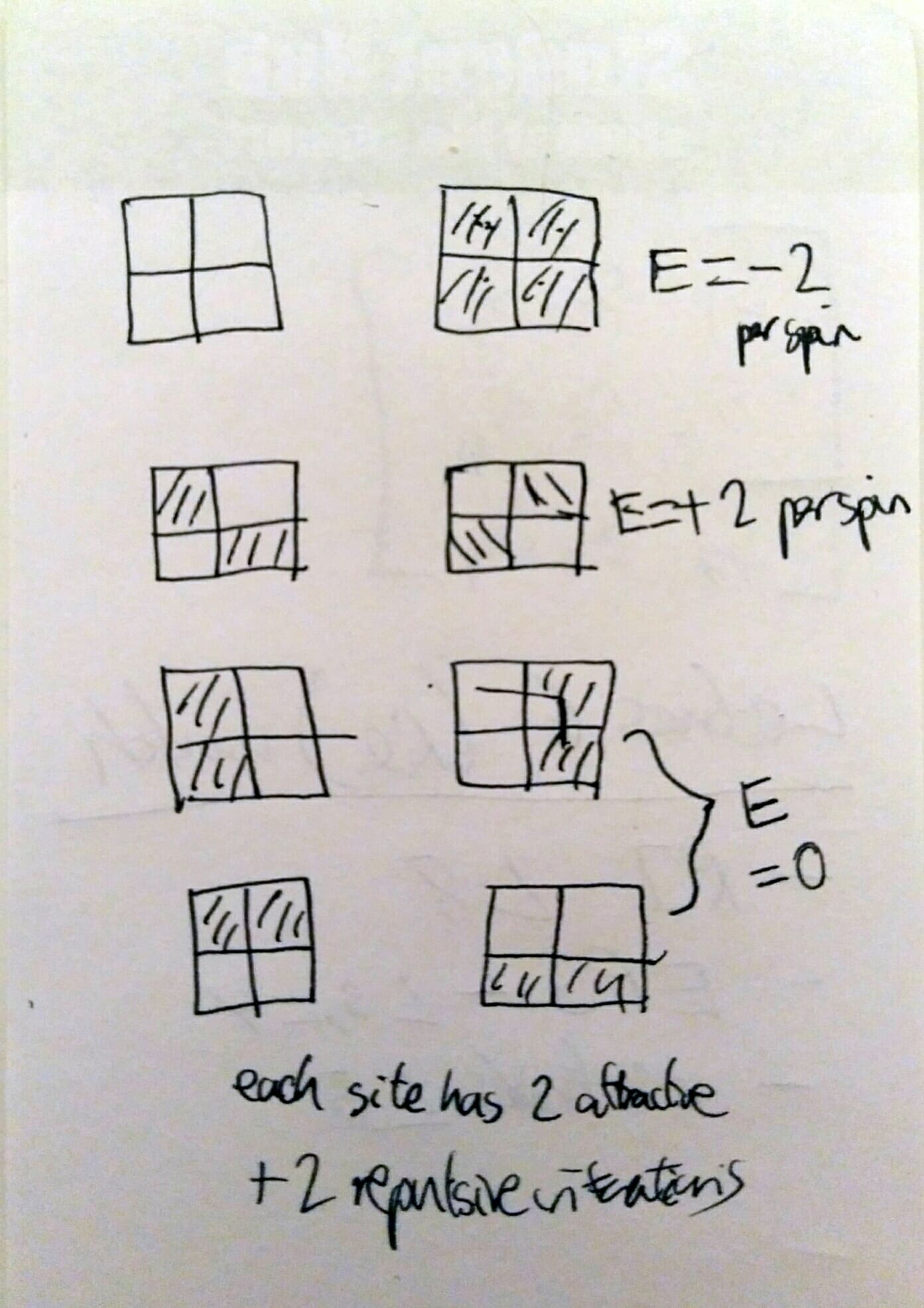
The magnetisations of these systems behaves quite differently depending on lattice size. For the lattices smaller than 16 x 16, the magnetisation starts out as a flat line with $⟨M⟩\approx 0$ that abruptly starts fluctuating with decreasing amplitude. These long range fluctuations, however, are not observed in the 16x16 and 32x32 systems, instead the magnetisation sharply drops at $T\approx 2.3$ and fluctuates around $⟨M⟩$ = 0, with a small amplitude. These fluctuations in magnetisation likely don't appear for the larger systems so strongly due to the larger lattice size.

Figure: Average energy/magnetisation vs. Temperature plots for 2x2, 4x4, 16x16 and 32x32 Ising Lattices (a. ,b. ,c. and d. respectively). As before the error bars are the standard deviations of the plotted means.

The error bars in the energies/magnetisations drastically decrease with increasing lattice size. As mentioned before, flipping a single spin in a large lattice has a small effect on the overall energy (especially so for energy per spin), hence the 'thermal' fluctuations in the system are much smaller (see the 'finalframe' plots in section 5).

Section 7: Determining the heat capacity

TASK: Derive Heat Capacity Expression

Given:

$C_V=\frac{\partial ⟨E⟩}{\partial T}$

And:

$⟨E⟩=\frac{1}{Z}\sum _{\alpha }E(\alpha )\exp (-\frac{E(\alpha )}{k_{B}T})=\frac{\sum _{\alpha }E(\alpha )\exp (-\frac{E(\alpha )}{k_{B}T})}{\sum _{\alpha }\exp (-\frac{E(\alpha )}{k_{B}T})}$

Using:

$C_V=\frac{\partial ⟨E⟩}{\partial T}=-\frac{1}{k_B{T}^2}\frac{\partial ⟨E⟩}{\partial \beta }$

$=-\frac{1}{k_B{T}^2}\frac{\partial }{\partial \beta }\left(\frac{\sum _{\alpha }E(\alpha )\exp (-E(\alpha )\beta )}{\sum _{\alpha }\exp (-E(\alpha )\beta )}\right)$

Applying Quotient Rule:

$=-\frac{1}{k_B{T}^2}\left[\frac{(\sum _{\alpha }\exp (-E^2(\alpha )\beta ))(\sum _{\alpha }(-1)E(\alpha )\exp (-E(\alpha )\beta ))-(\sum _{\alpha }E(\alpha )\exp (-E(\alpha )\beta ))(\sum _{\alpha }(-1)E(\alpha )\exp (-E(\alpha )\beta ))}{{(\sum _{\alpha }\exp (-E(\alpha )\beta ))}^2}\right]$

$=\frac{1}{k_B{T}^2}[\frac{\sum _{\alpha }{E}^2(\alpha )\exp (-E(\alpha )\beta )}{\sum _{\alpha }\exp (-E(\alpha )\beta )}-{\left(\frac{\sum _{\alpha }E(\alpha )\exp (-E(\alpha )\beta )}{\sum _{\alpha }\exp (-E(\alpha )\beta )}\right)}^2]$

From the definitions of $⟨E⟩,⟨E^2⟩$and $\mathrm{V}\mathrm{a}\mathrm{r}(E)=⟨E^2⟩-⟨E{⟩}^2$:

$C_V=\frac{1}{k_B{T}^2}[⟨E^2⟩-⟨E{⟩}^2]=\frac{\mathrm{V}\mathrm{a}\mathrm{r}(E)}{k_B{T}^2}$

As required. This formula can then be used to calculate the heat capacity from $⟨E⟩$ and $⟨E^2⟩$, which are properties already returned by the simulation.

TASK: Write a Python script to make a plot showing the heat capacity versus temperature for each of your lattice sizes from the previous section. You may need to do some research to recall the connection between the variance of a variable, $\mathrm{V}\mathrm{a}\mathrm{r}[X]$, the mean of its square $⟨X^2⟩$, and its squared mean ${⟨X⟩}^2$. You may find that the data around the peak is very noisy — this is normal, and is a result of being in the critical region. As before, use the plot controls to save your PNG image of your plot and attach this to the report.

The plots were generated in a Jupyter notebook. The data was loaded in with the following code:

sizes =np.array([2,4,8,16,32])
spins = sizes**2
#temporararily assigned the size, replaced by list of values extracted from the loaded.dat file
temps=[2,4,8,16,32]
ener=[2,4,8,16,32]
enersq=[2,4,8,16,32]
mag=[2,4,8,16,32]
magsq=[2,4,8,16,32]
# i is index, n is size
for i,n in enumerate(sizes):
    #transposes the array created by np.loadtext so the elements in the transposed array are arrays of the corresponding variables 
    temps[i],ener[i],enersq[i],mag[i],magsq[i] = np.transpose(np.loadtxt('run_data/{size}x{size}.dat'.format(size=n)))

Hence, for example, calling ener[4] returns the list of energies outputted by ILtempraturerange.py for the 32 by 32 lattice. Simialr code imported the C++ data (next section). The code used to calculate the vaiances of each variable for each system is:

varen=[]
varenC=[]
varmag=[]
varmagC=[]
for i, n in enumerate(sizes):
    varen.append((enersq[i]-ener[i]**2))
    varenC.append((enersqC[i]-enerC[i]**2))
    varmag.append(magsq[i]-mag[i]**2)
    varmagC.append(magsqC[i]-magC[i]**2)
# heat capacity of the python data. heat_cap[0] is for 2 by 2 etc. Calculated from the derived eqn.
heat_cap = np.array(varen)/np.array(temps)**2

The heat capacities (along with those of the C++data) were then plotted and saved with:

for i, n in enumerate(sizes):
    fig = plt.figure(figsize=(10,5))
    cap_plot = fig.add_subplot(1,1,1)
    cap_plot.set_title('$C_v$ vs. $T$ for {}x{} Lattice'.format(n,n))
    #heat capacity calculated according to derived eqn.
    cap_plot.plot(temps[i],varen[i]/temps[i]**2/n**2,label='Python Data')
    #Cdata multiplied by number of spins, as varenC is per spin squared
    cap_plot.plot(tempsC[i],varenC[i]/tempsC[i]**2*n**2,label='C++ Data')
    fig.legend()
    cap_plot.set_xlabel(r'$T$',fontsize=15)
    cap_plot.set_ylabel(r'$C_v$',fontsize=15)
    cap_plot.set_xlim(0,5.1)
    #cap_plot.set_ylim(0,0.5)
    plt.savefig('figs_for_rep/heat_cap_{}x{}'.format(n,n))
plt.show()

The heat capacity vs. temperature of several differently sized Ising lattices. $C_V$ is plotted per spin.

Plotting the heat capacity (per spin) shows that the heat capacity peaks gets narrower and taller with increasing lattice size and shifts slightly(due to the small differences in the Curie Temperature between the systems). As the lattice size tends to infinity, the phase transition becomes first order and the heat capacity diverges at $T=T_C$, as an infinitely long and narrow peak. The heat capacity plots generated from the python simulation correspond quite nicely with the C++ data, which comes from a higher quality simulation. The only exception is the 2 x 2 plot, which seems to underestimate the peak heat capacity.

Section 8: Determining the Curie Temperature

The Curie Temperature of a finite sized lattice can be related to that of an infinite lattice by:

$T_{c,L}=\frac{A}{L}+T_{c,infty}$

Comparing to C++ Data

TASK: A C++ program has been used to run some much longer simulations than would be possible on the college computers in Python. You can view its source code here if you are interested. Each file contains six columns: $T,E,E^2,M,M^2,C$ (the final five quantities are per spin), and you can read them with the NumPy loadtxt function as before. For each lattice size, plot the C++ data against your data. For one lattice size, save a PNG of this comparison and add it to your report — add a legend to the graph to label which is which. To do this, you will need to pass the label="..." keyword to the plot function, then call the legend() function of the axis object (documentation here).

The 16 by 16 lattice is compared with the results of the C++ program in the figure above. They appear to produce fairly similar results, except the C++ data shows more oscillations in the phase transition on the magnetisation plot and a much smoother line after phase transition. The heat capacities also appear to adopt a similar shape and peak, however, the far lower temperature resolution of the python code makes its heat capacity plot a lot spikier near the Curie temperature. The code for plotting the magnetisation vs. T and energy vs. T plots was:

for i, n in enumerate(sizes):
    fig = plt.figure(figsize=(10,10))
    
    
    
    mag_plot = fig.add_subplot(2,1,2)
    mag_plot.errorbar(temps[i],mag[i]/n**2,label='Python Data',yerr = np.array(varmag[i])**0.5/n**2,errorevery=3,ecolor='purple',color='blue')
    mag_plot.errorbar(tempsC[i], magC[i],label='C++ Data',yerr = np.array(varmagC[i])**0.5,errorevery=10,ecolor='pink',color='red')
    plt.setp(mag_plot.get_xticklabels(), fontsize=12)
    mag_plot.tick_params(axis='y',labelsize=12)
    #mag_plot.set_title(r'$\left<M\right>$ vs. $T$ of {}x{} Lattice'.format(n,n))
    mag_plot.set_ylabel(r'$\left<M\right>$per spin')
    mag_plot.set_xlabel(r'$T$')
    mag_plot.set_xlim(0,5.1)
    
    ener_plot = fig.add_subplot(2,1,1,sharex = mag_plot)
    ener_plot.set_title(r'$ \left< E \right> $ and $\left<M\right>$ vs. $T$ of {}x{} Lattice'.format(n,n))
    ener_plot.errorbar(temps[i],ener[i]/n**2,label='Python Data',yerr = np.array(varen[i])**0.5/n**2,errorevery=3,ecolor='purple',color='blue')
    ener_plot.errorbar(tempsC[i],enerC[i],label='C++ Data',yerr = np.array(varenC[i])**0.5,errorevery=10,ecolor='pink',color='red')
    plt.setp(ener_plot.get_xticklabels(), visible=False)
    ener_plot.tick_params(bottom=True)
    ener_plot.legend(loc='upper left')
    ener_plot.tick_params(axis='y',labelsize=12)
    ener_plot.set_ylabel(r'$\left<E\right>$per spin')
    
    fig.subplots_adjust(hspace = 0.1)
    plt.savefig('figs_for_rep/{}x{}_ccompare.png'.format(n,n))
plt.show()

Which simply plots the data imported into the Jupyter notebook via the code described in the previous section.

Polynomial Fitting

TASK: write a script to read the data from a particular file, and plot C vs T, as well as a fitted polynomial. Try changing the degree of the polynomial to improve the fit — in general, it might be difficult to get a good fit! Attach a PNG of an example fit to your report. TASK: Modify your script from the previous section. You should still plot the whole temperature range, but fit the polynomial only to the peak of the heat capacity! You should find it easier to get a good fit when restricted to this region.

The fitting in this sections was also carried out via a Jupyter notebook, instead of a separate script. The data was imported as described in the previous section, then the following code was used to generate the fit, for example for 2x2:

Tmin = np.min(temps[0])
Tmax = np.max(temps[0])
T_range = np.linspace(Tmin, Tmax, 1000) #generate 1000 evenly spaced points between T_min and T_max 

fit2 = np.polyfit(temps[0],heat_cap[0], 12) # fit a n order polynomial
fitted_C_values2=np.polyval(fit2, T_range) # use the fit object to generate the corresponding values of C

fig=plt.figure(figsize=(15,10))
#plt.figsize(15,10)
plt.plot(T_range,fitted_C_values2/4)
plt.plot(temps[0],heat_cap[0]/4,ls='',marker='o')
plt.xlabel(r'${T}$',fontsize=15)
plt.ylabel(r'$C_v$',fontsize=15)
plt.savefig('2x2_heatcap_whole_fit')
plt.xlim(0,5.1)
plt.show()

The fits for the other lattice sizes are plotted/ calculated by replacing variables that refer to system size(i.e. heat_cap[i] etc.). Writing a single script to run that takes a filename as an input would have been faster to implement, but it was more convenient to be able to tweak the order of the polynomial and replot on the fly to test different fits for different lattice sizes.

Example fit for the heat capacity of the 8 by 8 lattice. Fitted to a polynomial of the order 18

Attempting to fit over the whole temperature range results in the fit requiring a very high order polynomial. This fit can be improved by fitting over a smaller temperature range around the peak. Fitting a smooth polynomial over the spiky peaks of the heat capacity plots for the 16x16 and 32x32 systems presented an issue, where fitting over the vertical height of the peak was tricky, as very few points lied in the higher regions; only the 'spikes'.

The code here is similar to when fitting over the whole range:

#lists of max and min temps of peak for all lattice sizes
Tminpeak = [1.0,1.6,1.7,1.8,1.8]
Tmaxpeak = [4.0,4.0,3.2,3.1,2.8]
peak_T = []
peak_C =[]
for i, n in enumerate(sizes):
    #Picks only heat capacity and temperature values corresponding to the peaks
    selection = np.logical_and(np.array(temps[i]) > Tminpeak[i], np.array(temps[i]) < Tmaxpeak[i])
    #generates a list of lists
    peak_T.append(temps[i][selection])
    peak_C.append(heat_cap[i][selection])

Selects the values of C and T which are considered to be in the peak, for all 5 lattice sizes. Then plotted by:

fit2_peak = np.polyfit(peak_T[0],peak_C[0], 6) # fit a third order polynomial
fitted_C_values2_peak=np.polyval(fit2_peak, peak_T[0])

fig=plt.figure(figsize=(15,10))
#plt.figsize(15,10)
plt.plot(peak_T[0],fitted_C_values2_peak/4)
plt.plot(temps[0],heat_cap[0]/4,ls='',marker='o')
plt.xlabel(r'${T}$',fontsize=15)
plt.ylabel(r'$C_v$',fontsize=15)
plt.savefig('fits/2x2_heatcap_peak_fit')
plt.xlim(0,5.1)
plt.ylim(0,0.5)
plt.show()

Determining Curie Temperature

TASK: find the temperature at which the maximum in C occurs for each datafile that you were given. Make a text file containing two columns: the lattice side length (2,4,8, etc.), and the temperature at which C is a maximum. This is your estimate of $T_C$ for that side length. Make a plot that uses the scaling relation given above to determine $T_{C,\mathrm{\infty }}$. By doing a little research online, you should be able to find the theoretical exact Curie temperature for the infinite 2D Ising lattice. How does your value compare to this? Are you surprised by how good/bad the agreement is? Attach a PNG of this final graph to your report, and discuss briefly what you think the major sources of error are in your estimate.

The Curie Temperatures were found and subsequently stored based on the fits over the peaks, from data from the Python code, using the following code:

#Data calculated already
fitted_C_peak_list = [fitted_C_values2_peak,fitted_C_values4_peak,fitted_C_values8_peak,fitted_C_values16_peak,fitted_C_values32_peak]

curie_Ts =[]

for i,n in enumerate(sizes):
    c_max = np.max(fitted_C_peak_list[i])
    curie_Ts.append(peak_T[i][fitted_C_peak_list[i]==c_max])
print(curie_Ts)

curie_data = np.column_stack((sizes,curie_Ts))
np.savetxt('curie_data.dat',curie_data)

The data outputted can be found here: Media:Ac5116 Curie data.dat

Using python data: Fitting $T_{C,L}$ vs. $1/L$ to a straight line gives values for the Curie temperature of the inifinte lattice and the gradient of the scaling relation.

The fitting of the Curie Points with lattice size

The gradient and intercepts were found to be (0.5978 ± 0.0855) K and (2.304 ± 0.0221) K, respectively. This suggests the Curie Temperature of the infinite lattice is $T_{C\mathrm{\infty }}\approx$ (2.30 ± 0.02) K. The theoretically determined value is $T_{C\mathrm{\infty }}=$2.269 K (https://en.wikipedia.org/wiki/Square-lattice_Ising_model). This gives a surprisingly good agreement, given how few data points( lattice sizes) were used to calculate the Curie temperature. Major sources of error in this number may arise from how well defined the maximum of the fit to the underlying peak in $C_V$ is; hard to tell for the 'spiky' heat capacities. This results in uncertainty about the location of the Curie temperature $T_{C,L}$. The use of the 2 x 2 system to determine the gradient and intercept of the scaling relation may be invalid as it is very far away from an infinite lattice.