Rep:3rd Y CMP:fgk17

3^rd year CMP comp lab

introduction to the Ising model

task 1

In the Ising model the lowest energy is given by equation 1:

$E=-DNJ$ $\text{equation 1}$

Where D is the number of dimensions, N is the total number of spins and J is a constant which controls the strength of interactions. This equation is derived from equation 2:

$E=\frac{1}{2}J\sum _i^N\sum _{jϵneighbours(i)}{s}_i{s}_j$ $\text{equation 2}$

Where $s_i$and $s_j$ are the spins of a lattice site and its adjacent lattice sites, and N is the total number of lattice sites. At the lowest possible energy state there are a total of 2 possible configurations with either all of the spins being $+1$or $-1$ this means that $s_i{s}_j$ will always be equal to 1. The summation of all these possible interactions will be twice the sum of all of the actual interactions as they are all counted twice, leading to the $\frac{1}{2}$ at the front of the equation. The total number of interactions is equal to the number of spins times the dimensionality, as for a 2D lattice each spin under goes 4 interactions, however when calculating the E these are all calculated twice leading to the total number of interactions to be DN.

As there are 2 different options for the spin of a lattice site the lowest energy state can either have all of the lattice sites having a spin of $+1$or $-1$ meaning that the lowest energy state has a multiplicity of 2. The entropy (S) of the lattice is calculated by equation 3, where $\mathrm{\Omega }$ is the multiplicity and $k_B$ is the Boltzmann constant:

$S=k_{B}ln(\mathrm{\Omega })$ $\text{equation 3}$

Entropy of the lowest energy state:

$S=1.38\times 10^{-23}ln(2)$

$S=9.57\times 10^{-24}J/K$

task 2

For a system that is in the lowest energy configuration and has dimensions $(D=3,N=1000)$ the energy can be calculated using equation 1:

$E=-DNJ=-3(1000)J=-3000J$

If one of the spins at random flips spontaneously the energy increases. This energy is calculated using equation 2.

In this system each spin under goes a total of 6 different interactions resulting in a total of 6000 interactions with 12 being between a $+1$ and $-1$ spin and the rest being between like spins meaning that ${\mathrm{\Sigma }}_i^N{\mathrm{\Sigma }}_j{s}_i{s}_j$ is:

$5988(1)(1)+12(1)(-1)=5976$

Which when substituted in to equation 2 gives:

$E=-1/2(5976)J=-2988J$

Therefore the total energy change due to the flip is

$\mathrm{\Delta }E=-3000J--2988J=12J$

The multiplicity of the state after the flip has occurred is 2000 due to there there being 2 different starting states with either all $+1or-1$ spins resulting in 2000 possible resulting arrangements.

$S=k_{B}ln(2000)=1.049\times 10^{-22}J/K$

The gain in entropy between the 2 states is:

$\mathrm{\Delta }S=1.049\times 10^{-22}-9.57\times 10^{-24}=9.533\times 10^{-23}J/K$

task 3

The total magnetisation(M) of a system is given by equation 4:

$M={\mathrm{\Sigma }}_i{s}_i$ $\text{equation 4}$

For a 1D lattice with 3 positive spins and 2 negative spins, by using equation 4 the magnetisation can be seen to be 1. For a 2D lattice with 13 positive spins and 12 negative spins, the overall magnetisation is 1.

If the Ising lattice discussed above is at absolute zero, all the spins are in the same direction as the enthalpic driving forces are dominant. This means that all of the spins will align, resulting in the magnetisation being either -1000 or 1000. However, if the temperature is raised above the Curie temperature, it is expected that the entropic driving force would dominate, meaning that the expected magnetisation would be around 0.

Calculating the energy and magnetisation

Task 4

energy() functions

def energy(self):
        "Return the total energy of the current lattice configuration."
        energy = 0.0
        for i in range(0,self.n_rows):
            for j in range(0,self.n_cols):#runs through all of the lattice sights 
                x=int(i)-1 #finds the lattice sight to the left
                y=int(j)-1 #finds the lattice sight above
         
                energy=energy-self.lattice[x,j]*self.lattice[i,j]-self.lattice[i,y]*self.lattice[i,j]   #calculate the energy of the lattice sights and then add them to the running total of the energy 
        # as only two of the interactions with each lattice sight are looked at the resulting energy dose not need to be divided by 2 
        return energy 

the value for J in equation 2 is assumed to be 1 at all times as we are working in reduced units where $J=k_B$

magnetisation() function

def magnetisation(self):
        "Return the total magnetisation of the current lattice configuration."
        magnetisation=0
        for i in range(0,self.n_rows):
            for j in range(0,self.n_cols):
                magnetisation=magnetisation+int(self.lattice[i,j]) #runs through all of the lattice sites and adds them together to get the total magnetisation 
        
        return magnetisation 

Task 5

figure 1: showing expected enrgies and magnetisation for a 4x4 lattice

figure 1 shows the results of the provided ILcheck.py file to check that the energy and magnetisation code is outputting the expected values, which is what is seen.

Introduction to Monte Carlo simulation

Task 6

For a system with 100 different spins there are 2 possible configurations for each spin meaning that the total number of possible configurations is $2^{100}$ which is the same as $1.268\times 10^{30}$ configurations. Therefore to get the average energy and magnetization they all need to be calculated individually. If a computer is able to calculate at a rate of $1\times 10^9$ configurations per second then the total lengh of time to calculate a single ${⟨M⟩}_T$ would be $1.268\times 10^{21}$ seconds.

The average energy and magnetisations are calculated by equations 5 and 6:

$⟨M{⟩}_T=\frac{1}{Z}\sum _{\alpha }M\left(\alpha \right)\exp \{-\frac{E\left(\alpha \right)}{k_{B}T}\}$ $\text{equation 5}$

$⟨E{⟩}_T=\frac{1}{Z}\sum _{\alpha }E\left(\alpha \right)\exp \{-\frac{E\left(\alpha \right)}{k_{B}T}\}$ $\text{equation 6}$

Task 7

As can be seen from above, to calculate the average energy at a specific temperature would take a long long time and the equations do not take into account which arrangement of spins are more likely at a specific temperature. This problem is solved by using the Monte Carlo method. The method works by starting with a completely randomised set of spins in a lattice, flipping one and seeing if either the overall energy decreases or if the energy increases. Then if the probability for the change in state is greater than or equal to a random number between 0 and 1, it is accepted otherwise it is rejected, and the process is repeated until the energy is stabilised, at which point the average energy is taken.

The Monte Carlo function is created as below:

 
def montecarlostep(self, T):
        # complete this function so that it performs a single Monte Carlo step and takes the variable temperature
        energy_old = self.energy() # the energy of the old state is saved so that it can be used to compare to
        #the following two lines are used to select the coordinates of the random spin which will be flipped
        random_i = np.random.choice(range(0, self.n_rows))
        random_j = np.random.choice(range(0, self.n_cols))
        self.lattice[random_i,random_j]=-self.lattice[random_i,random_j]   #spin flipped 
        energy_new=self.energy() #energy of the new lattice calculated
        D_energy=energy_new-energy_old # difference in energies 
                   
        #the following line chooses a random number in the rang [0,1)
        random_number = np.random.random()
        
        self.n_cycles=self.n_cycles+1 #the cycle counter is updated 
        # if the change in energy is grater than zero and the random number which has been generated is grater than the Boltzmann factor the lattice is returned to the initial state
        if D_energy>0 and random_number>np.e**(-(D_energy)/T):
            self.lattice[random_i,random_j]=-self.lattice[random_i,random_j]

        # the sum of the energies and the magnetisations and both of there squares is updated only after 20000 cycles as this gives enables a better estimate of the energies to be calculated 
        if self.n_cycles>20000:
            self.E=self.E+self.energy()
            self.E2=self.E2+self.energy()**2
            self.M=self.M+self.magnetisation()
            self.M2=self.M2+self.magnetisation()**2
        #energy is in units of k_B
        return self.energy(), self.magnetisation()

The statistics function is defined as follows so as to generate <E>, <E^2>, <M>, <M^2> and the step count

def statistics(self):
        # complete this function so that it calculates the correct values for the averages of E, E*E (E2), M, M*M (M2), and the step count and returns them
        n=self.n_cycles #step count
        E=self.E/(self.n_cycles-20000) #avarage energy after 20000 steps
        E2=self.E2/(self.n_cycles-20000) #avarage energy squared after 20000 steps
        M=self.M/(self.n_cycles-20000) #avarage magnetisation after 20000 steps
        M2=self.M2/(self.n_cycles-20000) #avarage magnetisation squared after 20000 steps
        
        
        return E, E2, M, M2, n

Task 8

figure 2: optimisation of an 8 by 8 lattice when T=1, due to the animation file not working properly the resulting values generated by the statistics function where not outputted

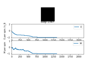
If the temperature is below the Curie temperature, it is expected that spontaneous magnetisation will occur. In figure 2 it can be can see that the Curie temperature is above 1.0 as the lattice tends to a constant magnetisation of -1 (all the spins are in the same direction) and the energy tends to -2 per spin (lowest energy state)

Accelerating the code

Task 8

When using 'for' statements to determine the energy and magnetisation, the time taken of the code to perform 2000 steps is 7.39323s $\pm 0.06948s$

Task 9

The program can be sped up by using the sum(), roll() and multiply() functions so that not every individual site in the lattice has to be checked individually against every other by using the roll function. It is possible to generate new lattices with the lattice sites moved either up or to the left by one. This can then be multiplied by the original lattice to get the spin interaction and then summed to get the total energy. The energy function

 
    def energy(self):
        "Return the total energy of the current lattice configuration."
        energy = np.sum(np.multiply(np.roll(self.lattice,1,axis=0),self.lattice))+np.sum(np.multiply(np.roll(self.lattice,1,axis=1),self.lattice)) #lattice is rolled once upwards and once to the left these are then multiplied by the ordinal lattice and summed so as to take in to account all of the interactions
        return -energy   #the negative of the energy is returned as the more favourable interaction is between like spins which output positive intergers

The magnetisation function

    
    def magnetisation(self):
        "Return the total magnetisation of the current lattice configuration."
        magnetisation=np.sum(self.lattice) #the sum of the elements of the lattice is taken
                        
        return magnetisation

Task 10

With the 'for' statements replaced as above, the run time for 2000 Monte Carlo steps is greatly decreased to 0.41342s $\pm 0.02199s$

The effect of temperature

Task 11

The provided ILfinalframe.py script was used to generate figures 3,4 and 5 which are of a 32 by 32 lattice at different temperatures

figure 3:32x32 lattice optimisation where T=1

figure 4:32x32 lattice optimisation where T=2

figure 5:32x32 lattice optimisation where T=5

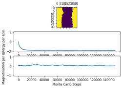
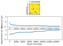
From these figures it can be seen that the energy per spin and magnetisation per spin both start a 0, however change rapidly within the first 20000 steps and then equilibrate (figure 4 does not show this in the magnetisation as it is near the Curie temperature and so takes longer to equilibrium). Because the starting values are not near the equilibrium values, the first 20000 steps are ignored so as to get more accurate values for the averages (these changes to the code can be seen in the Montecarlostep and statistics functions above).

Task 12

Average energy and magnetisation for different lattice sizes for T=0.25 to 5

2x2	4x4	8X8
16x16	32x32

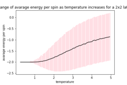
The data is generated using a modified version of the provided ILtemperature.py file and the error bars were calculated by taking the square root of the variance per spin. The code for modified version of the ILtemperature.py file is below:

from matplotlib import pylab as pl
import numpy as np

n_rows = 2 #number of rows in the lattice
n_cols = 2 #number of collums
il = IsingLattice(n_rows, n_cols)
il.lattice = np.ones((n_rows, n_cols))
spins = n_rows*n_cols #number of lattice sites
runtime = 100000
times = range(runtime) #number of steps run
temps = np.arange(0.25, 5, 0.05) #range of temperatures and interval size
energies = []
magnetisations = []
energysq = []
magnetisationsq = []
Eerr=[]
Merr=[]

for t in temps: #calles every number in the list of temperatures
    for i in times: #runs through each step in the cycle 
        
        energy, magnetisation = il.montecarlostep(t) #outputs the energy after each step
    aveE, aveE2, aveM, aveM2, n_cycles = il.statistics() #collects the energy at the end of each run of an individual temperature 
    energies.append(aveE) #compiles a list of energies
    energysq.append(aveE2) #compiles a list of energies squared
    magnetisations.append(aveM) #compiles a list of magnetisations
    magnetisationsq.append(aveM2) #compiles a list of magnetisations squared 
    Eerr.append(abs(aveE**2-aveE2)**0.5) # calculates erro in the energies
    Merr.append(abs(aveM**2-aveM2)**0.5) #calcualates error in the magnetisation 
    
    #reset the IL object for the next cycle
    il.E = 0.0
    il.E2 = 0.0
    il.M = 0.0
    il.M2 = 0.0
    il.n_cycles = 0
    
  #creates 2 plots one for energy and on for magnetisation   
fig = pl.figure()
enerax = fig.add_subplot(2,1,1)
enerax.set_ylabel("Energy per spin")
enerax.set_xlabel("Temperature")

magax = fig.add_subplot(2,1,2)
magax.set_ylabel("Magnetisation per spin")
magax.set_xlabel("Temperature")

enerax.plot(temps, np.array(energies)/spins, color='black') #plots average energy per spin vs temp 
enerax.errorbar(temps, np.array(energies)/spins,yerr=np.array(Eerr)/spins, color='pink',linestyle='') #plots error in the energy per spin vs temp

magax.plot(temps, np.array(magnetisations)/spins,color='black')#plots average magnetisation per spin vs temp 
magax.errorbar(temps, np.array(magnetisations)/spins,yerr=np.array(Merr)/spins,color='pink',linestyle='')#plots error in the mgnetisation per spin vs temp
pl.show()
#saves a data file containing temperature, energy, energy squared, magnetisatio, magnetisation squared
final_data = np.column_stack((temps, energies, energysq, magnetisations, magnetisationsq))
np.savetxt("4x4.dat", final_data)

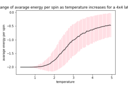
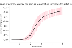
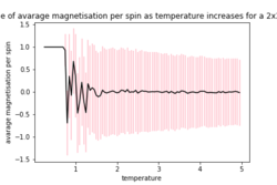
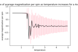
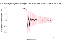
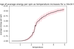
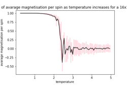
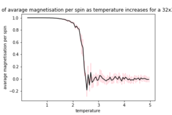
As the temperature increases the average energy also increases (those shown in the table are the average energy per spin) and goes through a point of inflection. Also as the temperature increases the average magnetisation per spin changes and goes from 1 down to 0 due to the en tropic driving forces. According the equation 7 the gradient of the average energy per spin vs temperature is the heat capacity.

The effect of system size

Task 13

figure 6,a:how energy per spin changes with temperature and lattice size

figure 6,b:how magnetisation per spin changes with temperature and lattice size

these graphs are plotted using the following code

x32=np.loadtxt('32x32.dat') #extracts the data from the data file
temp32=x32[:,0] #extracts the temperatures as a list from the data
E32=x32[:,1] #extracts the average energies from the data  
EE32=x32[:,2] #extracts the average square of the energies from the data 
M32=x32[:,3] #extracts the average magnetisation from the data
MM32=x32[:,4] #extracts the average square of the magnetisations from the data 
varE32=(np.array(EE32)-np.array(E32)**2)/(32*32) #calculates the variance of the energies per spin
varM32=(np.array(MM32)-np.array(M32)**2)/(32*32) #calculates the variance of the magnetisation per spin
Cv32=heat_capacity(temp32,varE32) #calculates the heat capacities


#plots the magnetisation per spin verses the temperature
pl.plot(temp32,M32/(32*32),label='32x32') #plots the magnetisation per spin verses the temperature
pl.xlabel('temperature')
pl.ylabel('magnetisation per spin')
pl.title('how magnetisation per spin varies as temperature increases for diffrent lattices sizes')
pl.legend()
pl.savefig('mag_vs_T.png') 
pl.show()

#plots the energy per spin verses the temperature
pl.plot(temp32,E32/(32*32),label='32x32')
pl.xlabel('temperature')
pl.ylabel('energy per spin')
pl.title('how energy per spin varies as temperature increases for diffrent lattices sizes')
pl.legend()
pl.savefig('en_vs_T.png')
pl.show()

As can be seen in figure 6a, the difference in the curve energy per spin vs temperature for 16x16 and 32x32 is small suggesting that they are both able to model the long range fluctuations. However there is still a slight in the magnetisation per spin vs temperature curve as seen in figure 6b, meaning that possibly the 16x16 lattice is not modelling them particularly well and a 32x32 lattice models them more accurately. If the lattice is to small the effect of one spin flipping is felt more greatly due to the periodic nature of the lattice if this is to small these spins can exert and effect on another. Both of these effects mean that the larger the lattice which is used the batter the prediction as it will model the long range fluctuation better and also eliminate the effect of the spin on its self as this decreases rapidly with distance.

Determining the heat capacity

Task 14

$C_v=\frac{\partial ⟨E⟩}{\partial T}\text{equation 7}$

$\text{show that}{C}_v=\frac{Var[E]}{k_B{T}^2}\text{equation 8}$

$\text{as previously stated }⟨E⟩=\frac{1}{z}\sum E{e}^{-\beta E}=-\frac{1}{z}\frac{\partial z}{\partial \beta }=-\frac{\partial ln(z)}{\partial \beta },\text{<mrow data-mjx-texclass="ORD">as</mrow>}\beta =\frac{1}{k_{B}T}\text{<mrow data-mjx-texclass="ORD">and</mrow>}z=e^{-\beta E}$

$\text{and as}\frac{\partial }{\partial T}=\frac{\partial \beta }{\partial T}\frac{\partial }{\partial \beta }=-\frac{1}{k_B{T}^2}\frac{\partial }{\partial \beta }$

$\text{<mrow data-mjx-texclass="ORD">then</mrow>}\frac{\partial ⟨E⟩}{\partial T}=\frac{\partial }{\partial T}(-\frac{1}{z}\frac{\partial z}{\partial \beta })=-\frac{1}{k_B{T}^2}\frac{\partial }{\partial \beta }(-\frac{1}{z}\frac{\partial z}{\partial \beta })=\frac{1}{k_B{T}^2}\left(\frac{{\partial }^{2}ln(z)}{\partial {\beta }^2}\right)$

$\text{<mrow data-mjx-texclass="ORD">as</mrow>}Var[E]=⟨E^2⟩-⟨E⟩\text{and as}⟨E^2⟩=\frac{1}{z}\sum E^2{e}^{-\beta E}=\frac{1}{z}\frac{{\partial }^{2}z}{\partial {\beta }^2}$

$\text{<mrow data-mjx-texclass="ORD">then</mrow>}Var[E]=⟨E^2⟩-⟨E{⟩}^2=\frac{1}{z}\frac{{\partial }^{2}z}{\partial {\beta }^2}-{(-\frac{1}{z}\frac{\partial z}{\partial \beta })}^2=\frac{1}{z}\frac{{\partial }^{2}z}{\partial {\beta }^2}-\frac{1}{z^2}{\left(\frac{\partial z}{\partial \beta }\right)}^2$

$\text{by expanding}\frac{\partial ⟨E⟩}{\partial T}-\frac{1}{k_B{T}^2}\frac{\partial }{\partial \beta }(-\frac{1}{z}\frac{\partial z}{\partial \beta })=\frac{1}{k_B{T}^2}(\frac{\partial \left(\frac{1}{z}\right)}{\partial \beta }\frac{\partial z}{\partial \beta }+\frac{1}{z}\frac{{\partial }^{2}z}{\partial {\beta }^2})=\frac{1}{k_B{T}^2}(-\frac{1}{z^2}{\left(\frac{\partial z}{\partial \beta }\right)}^2+\frac{1}{z}\frac{{\partial }^{2}z}{\partial {\beta }^2})=\frac{1}{k_B{T}^2}(⟨E^2⟩-⟨E⟩)\text{as seen above}$

$\text{therefore}\frac{\partial ⟨E⟩}{\partial T}=\frac{Var[E]}{k_B{T}^2}=C_v$

$\text{this also shows that}\frac{{\partial }^{2}ln(z)}{\partial {\beta }^2}=\frac{Var[E]}{k_B{T}^2}$

Task 15

figure 7: plot of heat capacity against temperature for different lattice sizes

The following function is used to generate the values for the heat capacity

def heat_capacity(T,var):
    "heat capacity form temperature an variance in units of k_B as E is already in unities of k_B"
    C=var/(T**2) 
    return C

This was then plotted using the plot function to give figure 7.

Locating the Curie temperature

Task 16

figure 10: comparisons between C++ data and self generated data for an 8x8 lattice

figure 8: comparisons between C++ data and self generated data for an 8x8 lattice

figure 9: comparisons between C++ data and self generated data for an 8x8 lattice

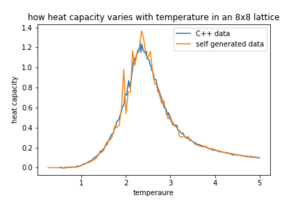
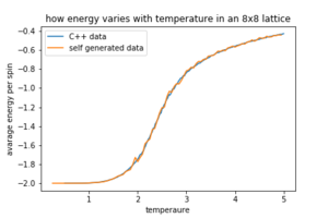
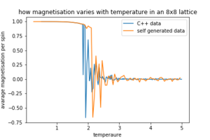
Figures 8,9 and 10 how how the data generated by our selves compares to the C++ data.

Task 17

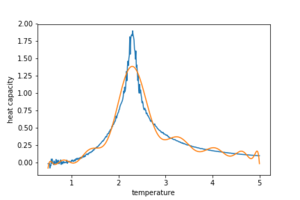
An initial fit for the C vs T data is generated by the code below so as to give figure 11 for a 32x32 lattice

figure 11: C vs T plot and fitted curve for 32x32 lattice

data = np.loadtxt('C32x32.dat')#C++ 32x32 generated data file is called
T = data[:,0] #get the first column
C = data[:,5] # get the sixth column


#a the polynomial is fitted to the data
fit = np.polyfit(T, C, 16) # fit a 16th order polynomial

#the maximum and minimum temperatures are found 
T_min = np.min(T)
T_max = np.max(T)
T_range = np.linspace(T_min, T_max, 1000) #generate 1000 evenly spaced points between T_min and T_max
fitted_C_values = np.polyval(fit, T_range) # use the fit object to generate the corresponding values of C

#data is plotted 
pl.plot(T,C,label='32x32') #data is plotted
pl.plot(T_range,fitted_C_values) #curve is plotted
pl.xlabel('temperature')
pl.ylabel('heat capacity')
pl.savefig('fk_polyfit_32_1st.png')
pl.show()

Task 18

figure 12: C vs T for a 32x32 lattice where the peak is fitted

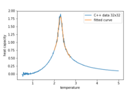
Figure 12 is generated using the code bellow where only the peak has been fitted

data = np.loadtxt('C32x32.dat')#C++ 32x32 generated data file is called
T = data[:,0] #get the first column
C = data[:,5] # get the sixth column

Tmin=2.0 #temperature around the peak
Tmax=2.75 #temperature around the peak

selection = np.logical_and(T > Tmin, T < Tmax) #select only the data around the peak of the curve
peak_T_values = T[selection]
peak_C_values = C[selection]

#data is fitted
fit2 = np.polyfit(peak_T_values, peak_C_values,9)#fit to the 10th order
T_min2 = np.min(peak_T_values)
T_max2 = np.max(peak_T_values)
T_range2 = np.linspace(T_min2, T_max2, 1000) #generate 1000 evenly spaced points between T_min and T_max
fitted_C_values2 = np.polyval(fit2, T_range2)

#data is plotted 
pl.plot(T,C,label='C++ data 32x32') #data is plotted
pl.plot(T_range2,fitted_C_values2,label='fitted curve') #curve is plotted
pl.xlabel('temperature')
pl.ylabel('heat capacity')
pl.legend()
pl.savefig('fk_polyfit_32_2st.png')
pl.show()

Task 19

figure 13: $\frac{1}{latticelength}\text{vs}{T}_{c,L}$

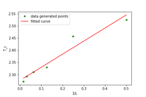
As the Curie temperature changes with the size of the lattice according to equation 7.

$T_{c,L}=\frac{A}{L}+T_{c,\mathrm{\infty }}\text{equation 8}$

where L is the lattice side length A is a constant $T_{c,L}$ is the Curie temperature for a given lattice size and $T_{c,\mathrm{\infty }}$ is the Curie temperature at infinity.

The curie temperature of an infinite lattice can be predicted by finding the y intercept of the graph in figure 13. The Curie temperature of an infinite lattice is predicted to be 2.27681069 through the use of the graph. that predicted in literature is 2.16667 to the second order. The value predicted by our model gives relatively good agreement. The major sources of error are likely to be due to the size of the lattices being looked at are small meaning that a by only flipping one spin there is a large effect on the average energy per spin. Also a grater number of montecarlo steps where used this would enable a better estimate of the energy to be calculated as the energy will be closer to the average energy for more of the steps.

final Isinglattic code

'''creating the Ising lattice model'''
import numpy as np

class IsingLattice:
# create statting values so as to keep runing totals of E, E^2, M, M^2 and n_cycles
    E = 0.0
    E2 = 0.0
    M = 0.0
    M2 = 0.0

    n_cycles = 1

    def __init__(self, n_rows, n_cols):
        self.n_rows = n_rows #number of rows in the lattise
        self.n_cols = n_cols #number of colums in the lattise
        self.lattice = np.random.choice([-1,1], size=(n_rows, n_cols)) #generate random spins for each lattice site

    
    def energy(self):
        "Return the total energy of the current lattice configuration."
        energy = np.sum(np.multiply(np.roll(self.lattice,1,axis=0),self.lattice))+np.sum(np.multiply(np.roll(self.lattice,1,axis=1),self.lattice)) #lattice is rolled once upwards and once to the left these are then multiplied by the ordinal lattice and summed so as to take in to account all of the interactions
        return -energy   #the negative of the energy is returned as the more favourable interaction is between like spins which output positive intergers
        
    def magnetisation(self):
        "Return the total magnetisation of the current lattice configuration."
        magnetisation=np.sum(self.lattice) #the sum of the elements of the lattice is taken
                        
        return magnetisation
    
    def montecarlostep(self, T):
        # complete this function so that it performs a single Monte Carlo step and takes the variable temperature
        energy_old = self.energy() # the energy of the old state is saved so that it can be used to compare to
        #the following two lines are used to select the coordinates of the random spin which will be flipped
        random_i = np.random.choice(range(0, self.n_rows))
        random_j = np.random.choice(range(0, self.n_cols))
        self.lattice[random_i,random_j]=-self.lattice[random_i,random_j]   #spin flipped 
        energy_new=self.energy() #energy of the new lattice calculated
        D_energy=energy_new-energy_old # difference in energies 
                   
        #the following line chooses a random number in the rang [0,1)
        random_number = np.random.random()
        
        self.n_cycles=self.n_cycles+1 #the cycle counter is updated 
        # if the change in energy is grater than zero and the random number which has been generated is grater than the Boltzmann factor the lattice is returned to the initial state
        if D_energy>0 and random_number>np.e**(-(D_energy)/T):
            self.lattice[random_i,random_j]=-self.lattice[random_i,random_j]

        # the sum of the energies and the magnetisations and both of there squares is updated only after 20000 cycles as this gives enables a better estimate of the energies to be calculated 
        if self.n_cycles>20000:
            self.E=self.E+self.energy()
            self.E2=self.E2+self.energy()**2
            self.M=self.M+self.magnetisation()
            self.M2=self.M2+self.magnetisation()**2
        #energy is in units of k_B
        #returnes energy and magentisation of resulting state
        return self.energy(), self.magnetisation()

    def statistics(self):
        # complete this function so that it calculates the correct values for the averages of E, E*E (E2), M, M*M (M2), and the step count and returns them
        n=self.n_cycles #step count
        E=self.E/(self.n_cycles-20000) #avarage energy after 20000 steps
        E2=self.E2/(self.n_cycles-20000) #avarage energy squared after 20000 steps
        M=self.M/(self.n_cycles-20000) #avarage magnetisation after 20000 steps
        M2=self.M2/(self.n_cycles-20000) #avarage magnetisation squared after 20000 steps
        
        #rerurnes E,E^2,M,M^2 and step number
        return E, E2, M, M2, n