Rep:3CMPks4817

TASK: Show that the lowest possible energy for the Ising model is E\ =\ -DNJ, where D is the number of dimensions and N is the total number of spins. What is the multiplicity of this state? Calculate its entropy.

The lowest possible energy configuration would have all the spins orientated in the same direction. Therefore all the spins would be either spin up or down.

Because the interactions are periodic the number of interactions for each spin would be 2 in every dimension. So if the lattice is 1D each spin would have 2 interactions. If the lattice is 2D each spin would have 4 interactions.

Moreover, the spins all being either s_i=s_j=1 or s_i=s_j=-1 hence s_i x s_j=1. So if you plug the interactions into the summationː

$\sum_{i}^{N} \sum_{j \in n e i g h b o u r s (i)} s_{i} s_{j}$

All the interactions would sum up to the total number of interactionsː 2ND.

If you plug the numbers into the full interaction energy equationː

$E = - \frac{1}{2} J \sum_{i}^{N} \sum_{j \in n e i g h b o u r s (i)} s_{i} s_{j}$

$E = - \frac{1}{2} J 2 N D$

$E = - J N D$

The multiplicity of the states is 2 as having all the spins being spin up or spin down would give you the same energy.

The total entropy can be calculated from the Boltzmann's equation for entropy, W being the multiplicity of the statesː

$S = k_{B} l n (W)$

$S = 1.38064852 \times 1 0^{- 23} \times l n (2)$

$S = 9.5699263 \times 1 0^{- 24}$

TASK: Imagine that the system is in the lowest energy configuration. To move to a different state, one of the spins must spontaneously change direction ("flip"). What is the change in energy if this happens (D=3,\ N=1000)? How much entropy does the system gain by doing so?

The lowest interaction energy for this system would beː

$E = - J N D$

$E = - J / t i m e s 1000 / t i m e s 3$

$E = - 3000 J$

If you flip one spin then there will be 12 interactions which give a negative interaction as each of the 6 neighbours gain a negative interaction (you add the interactions to the negative energy making it higher in energy) and the spin which flipped direction gains 6 negative interactionsː

$Δ E = 12 J$

So the new state would have an energy of

$E = - 3000 J + 12 J$

$E = - 2988 J$

The change in entropy would have the multiplicity change from 2 states to 2000 as you either start with all the states up and have 1000 possibilities to spin flip or you start with all the states down and have 1000 possibilities to spin flip.

The entropy would therefore beː

$S = k_{B} l n (W)$

$S = 1.38064852 \times 1 0^{- 23} \times l n (2000)$

$S = 1.0494175 \times 1 0^{- 22}$

Therefore the energy goes up in value (is more destabilised) but the entropy increases by 2 whole magnitudes.

TASK: Calculate the magnetisation of the 1D and 2D lattices in figure 1. What magnetisation would you expect to observe for an Ising lattice with D = 3,\ N=1000 at absolute zero?

The magnetization for the 1D lattice is 1 and the magnetisation for the 2D lattice is also 1 since the sums of the +1 and -1 spins both give this value.

1Dː $M = \sum_{i} s_{i}$ $M = 3 - 2$ $M = 1$

2Dː $M = \sum_{i} s_{i}$ $M = 13 - 12$ $M = 1$

The magnetisation for a D=3, N=1000 lattice at absolute 0 would have the lowest energy state dominate and therefore have all the spins be in the same direction adding up to either 1000 or -1000.

TASK: complete the functions energy() and magnetisation(), which should return the energy of the lattice and the total magnetisation, respectively. In the energy() function you may assume that J=1.0 at all times (in fact, we are working in reduced units in which J=k_B, but there will be more information about this in later sections). Do not worry about the efficiency of the code at the moment — we will address the speed in a later part of the experiment.

   def energy(self):
       "Return the total energy of the current lattice configuration."
       energy = 0.0
       i=0
       j=0
       #uses % so when the values are equal to the end of the lattice (array index+1=collumn or row) it returns to the initial index 
        of 0, hence multiplies it by the periodic neighbour
       #runs through i rows and then j collumns to calculate energies
       while i<self.n_rows:
           while j<self.n_cols:
               energy=energy-self.lattice[i,j]*self.lattice[(i+1)%self.n_rows,j]-self.lattice[i,j]*self.lattice[i,(j+1)%self.n_cols]
               j=j+1
           j=0
           i=i+1               
       return energy

   def magnetisation(self):
       "Return the total magnetisation of the current lattice configuration."
       magnetisation=0
       #runs through all values in array first with rows i then collumns j and adds them together
       for i in self.lattice:
           for j in i:
               magnetisation=magnetisation+j
       return magnetisation

TASK: Run the ILcheck.py script from the IPython Qt console using the command

TASK: How many configurations are available to a system with 100 spins? To evaluate these expressions, we have to calculate the energy and magnetisation for each of these configurations, then perform the sum. Let's be very, very, generous, and say that we can analyse 1\times 10^9 configurations per second with our computer. How long will it take to evaluate a single value of \left\langle M\right\rangle_T?

The number of configurations would be 2¹⁰⁰ and the time it would take would beː

$\frac{2^{100}}{1 0^{9}} = 1.267 \times 1 0^{21} s e c o n d s$

TASK: Implement a single cycle of the above algorithm in the montecarlocycle(T) function. This function should return the energy of your lattice and the magnetisation at the end of the cycle. You may assume that the energy returned by your energy() function is in units of k_B! Complete the statistics() function. This should return the following quantities whenever it is called: <E>, <E^2>, <M>, <M^2>, and the number of Monte Carlo steps that have elapsed.

   def montecarlostep(self, T):
      
       # complete this function so that it performs a single Monte Carlo step
       energy = self.energy()
       magnet=self.magnetisation()
       #the following two lines will select the coordinates of the random spin for you
       random_i = np.random.choice(range(0, self.n_rows))
       random_j = np.random.choice(range(0, self.n_cols))
       self.lattice[random_i, random_j]=self.lattice[random_i, random_j]*-1 #changes the spin of the random coordinate
       #the following line will choose a random number in the rang e[0,1) for you
       random_number = np.random.random()
       self.n_cycles=self.n_cycles+1 #keeps track of number of steps

       E1=self.energy()
       de=E1-energy
       if de>0 and random_number>np.exp(-1*(E1-energy)/(T)):
           self.lattice[random_i, random_j]=self.lattice[random_i, random_j]*-1 #if the lattice is not of lower energy and the probability doesn't allow it to occur the spin of that randomely changed coordinate should be reset back to 0
       if self.n_cycles>20000:
           self.E=(self.E+self.energy())
           self.E2=(self.E2+self.energy()**2)
           self.M=(self.M+self.magnetisation())
           self.M2=(self.M2+self.magnetisation()**2)#calculates E, E2, M, M2 for use in statistics
      #recalculate self energy and self magnetisation again once the new lattice has been chosen based on whether it is lower E
       return(self.energy(),self.magnetisation())
      
      
      
   def statistics(self):
       # complete this function so that it calculates the correct values for the averages of E, E*E (E2), M, M*M (M2), and returns 
         them
       #calculated the sums in montecarlo step now just the averages
      
       n=self.n_cycles
       E=(self.E)/(self.n_cycles)
       E2=(self.E2)/(self.n_cycles)
       M=(self.M)/(self.n_cycles)
       M2=(self.M2)/(self.n_cycles)
          
      
       return(E,E2,M,M2,n)

TASK: If T < T_C, do you expect a spontaneous magnetisation (i.e. do you expect \left\langle M\right\rangle \neq 0)? When the state of the simulation appears to stop changing (when you have reached an equilibrium state), use the controls to export the output to PNG and attach this to your report. You should also include the output from your statistics() function.

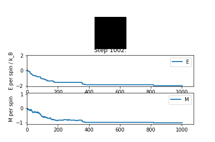
Yes you expect a spontaneous magnetisation when you run the stimulation - this is because the temperature is lower than the critical temperature or the curie temperature therefore the energy effects dominate and the spins get preferentially orientated in the same direction. When you have reached the equilibrium state the spins are either at a max or min (depending on whether they are all spin up or spin down) and the energies are at a min.

TASK: Use the script ILtimetrial.py to record how long your current version of IsingLattice.py takes to perform 2000 Monte Carlo steps. This will vary, depending on what else the computer happens to be doing, so perform repeats and report the error in your average!

Run Timesː 2.9668559 s , 2.8756327000000113 s , 2.8563893999999834 s , 2.8704408999999487 s, 2.890054399999997 s, 2.8774457000000098 s, 2.899158399999976 s, 2.9200945999999703 s , 3.6873911000000135 s, 2.8700606999999536 s

Averageː 2.971352379999986 s

Standard Deviationː 0.2405869279229322 s

TASK: Look at the documentation for the NumPy sum function. You should be able to modify your magnetisation() function so that it uses this to evaluate M. The energy is a little trickier. Familiarise yourself with the NumPy roll and multiply functions, and use these to replace your energy double loop (you will need to call roll and multiply twice!).

   def energy(self):
       "Return the total energy of the current lattice configuration."
       #creates a rolled over array of all the values moved to the left then all the values moved up one and multiplies them by the 
        original- so original multiplied by left value and up value withought a worry of running out of lattice because it rolls over
       energy=-np.sum(np.multiply(self.lattice, np.roll(self.lattice, 1, 1)))-np.sum(np.multiply(self.lattice, np.roll(self.lattice, 1, 0)))      
            
      
       return energy

   def magnetisation(self):
       "Return the total magnetisation of the current lattice configuration."
       #just sums through all the vallues in the 2D array immediately, rather than using an if statement
       magnetisation=np.sum(self.lattice)
       
       return magnetisation

TASK: Use the script ILtimetrial.py to record how long your new version of IsingLattice.py takes to perform 2000 Monte Carlo steps. This will vary, depending on what else the computer happens to be doing, so perform repeats and report the error in your average!

Run Timesː 0.3054809999994177 s, 0.2789596000002348 s, 0.2797293000003265 s, 0.27966940000078466 s, 0.281343000000561 s, 0.27697489999991376 s, 0.2813248999991629 s, 0.2809349999988626 s, 0.2788835999999719 s, 0.2795488000010664 s

Averageː 0.28228495000003023 s

Standard Deviationː 0.007831799265619254 s

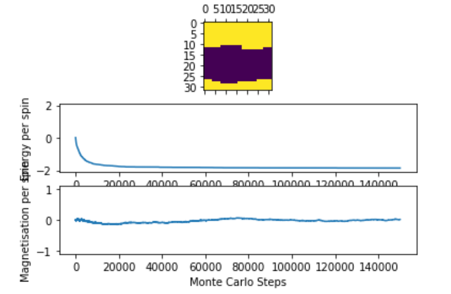
TASK: The script ILfinalframe.py runs for a given number of cycles at a given temperature, then plots a depiction of the final lattice state as well as graphs of the energy and magnetisation as a function of cycle number. This is much quicker than animating every frame! Experiment with different temperature and lattice sizes. How many cycles are typically needed for the system to go from its random starting position to the equilibrium state? Modify your statistics() and montecarlostep() functions so that the first N cycles of the simulation are ignored when calculating the averages. You should state in your report what period you chose to ignore, and include graphs from ILfinalframe.py to illustrate your motivation in choosing this figure.

The period chosen past the equilibration point was 20000. The lower the temperature the longer the time taken to equilibrate and the larger the lattice the longer it takes to equilibrate hence running 32x32 at 0.25 K gave us this energy graph and around 20000 the energy was already equilibrating.

The code used to fix this can be seen bellow:

       def statistics(self):
       # complete this function so that it calculates the correct values for the averages of E, E*E (E2), M, M*M (M2), and returns them
       
       if self.n_cycles>20000:
           E=(self.E+self.energy())/(self.n_cycles-20000)
           E2=(self.E2+self.energy()**2)/(self.n_cycles-20000)
           M=(self.M+self.magnetisation())/(self.n_cycles-20000)
           M2=(self.M2+self.magnetisation()**2)/(self.n_cycles-20000)
           
       else: 
          E = 0.0
          E2 = 0.0
          M = 0.0
          M2 = 0.0
       return(E,E2,M,M2, self.n_cycles)

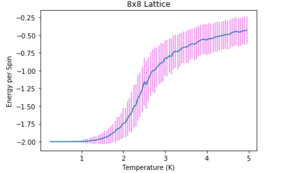
TASK: Use ILtemperaturerange.py to plot the average energy and magnetisation for each temperature, with error bars, for an 8\times 8 lattice. Use your intuition and results from the script ILfinalframe.py to estimate how many cycles each simulation should be. The temperature range 0.25 to 5.0 is sufficient. Use as many temperature points as you feel necessary to illustrate the trend, but do not use a temperature spacing larger than 0.5. The NumPy function savetxt() stores your array of output data on disk — you will need it later. Save the file as 8x8.dat so that you know which lattice size it came from.

See bellow

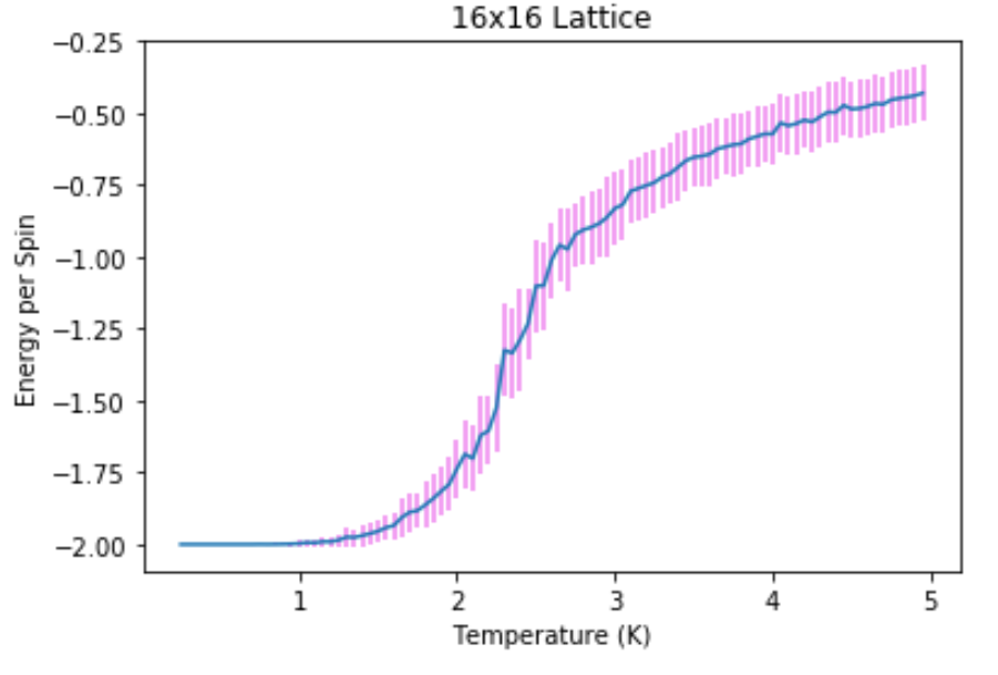
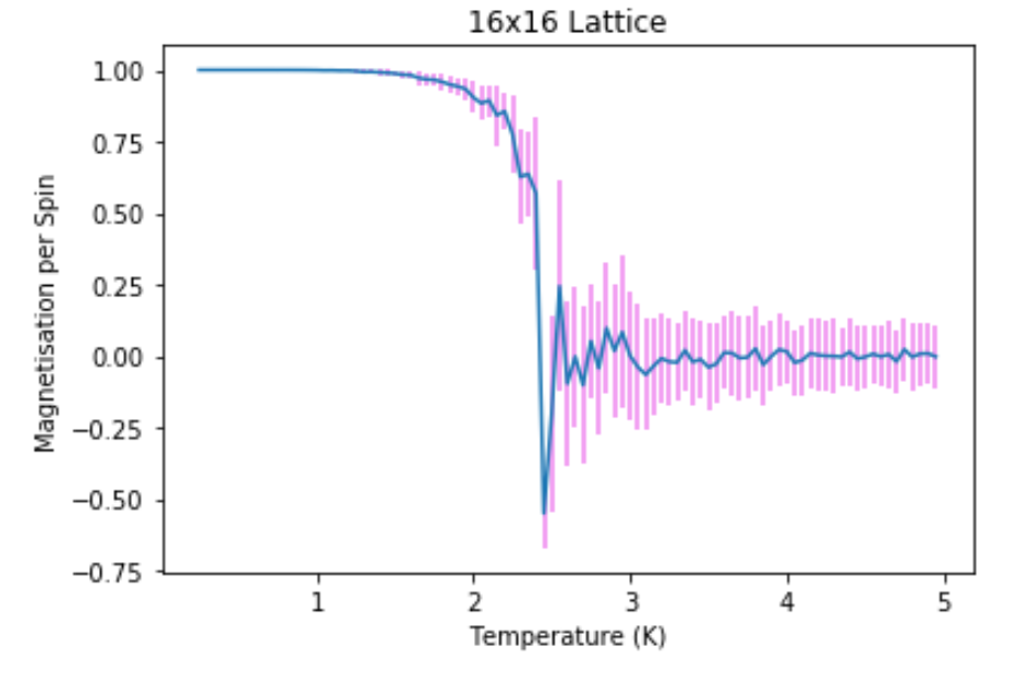
TASK: Repeat the final task of the previous section for the following lattice sizes: 2x2, 4x4, 8x8, 16x16, 32x32. Make sure that you name each datafile that your produce after the corresponding lattice size! Write a Python script to make a plot showing the energy per spin versus temperature for each of your lattice sizes. Hint: the NumPy loadtxt function is the reverse of the savetxt function, and can be used to read your previously saved files into the script. Repeat this for the magnetisation. As before, use the plot controls to save your a PNG image of your plot and attach this to the report. How big a lattice do you think is big enough to capture the long range fluctuations?

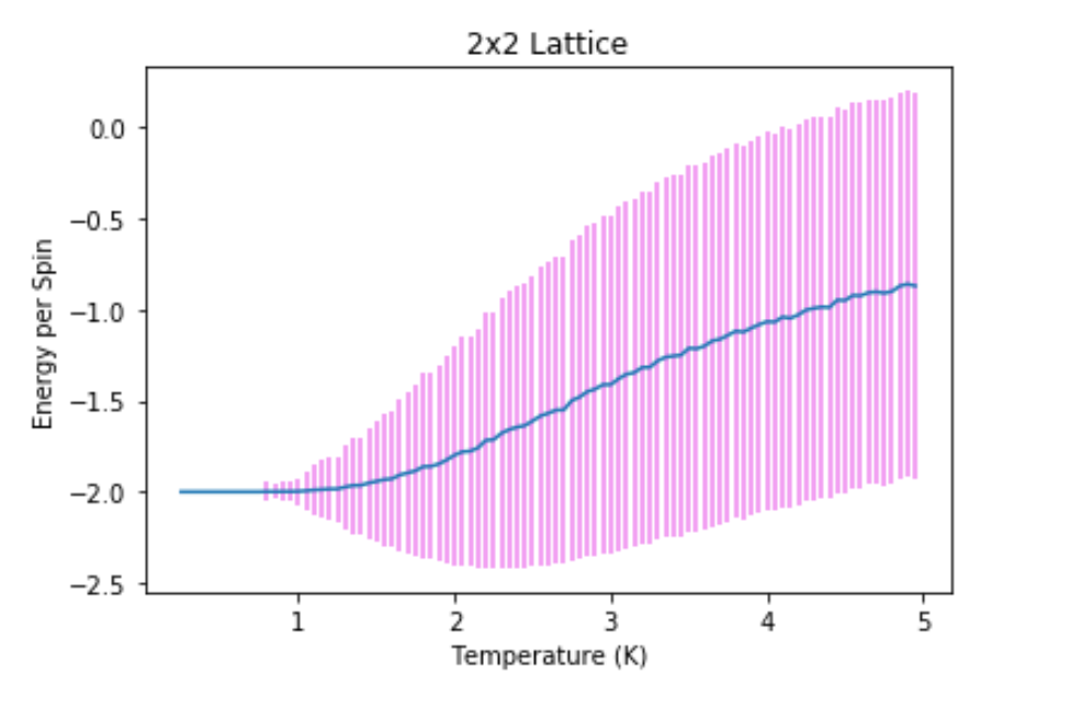
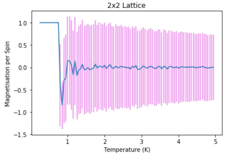
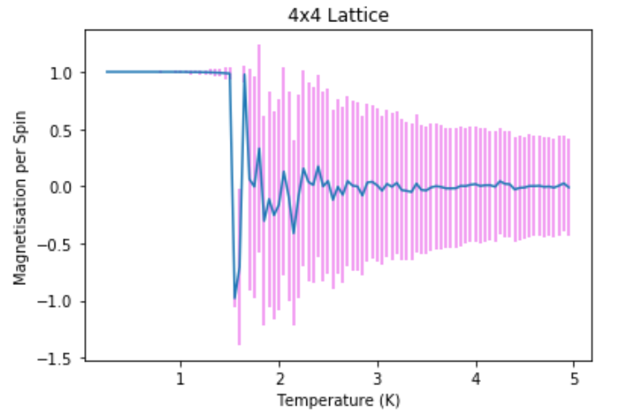
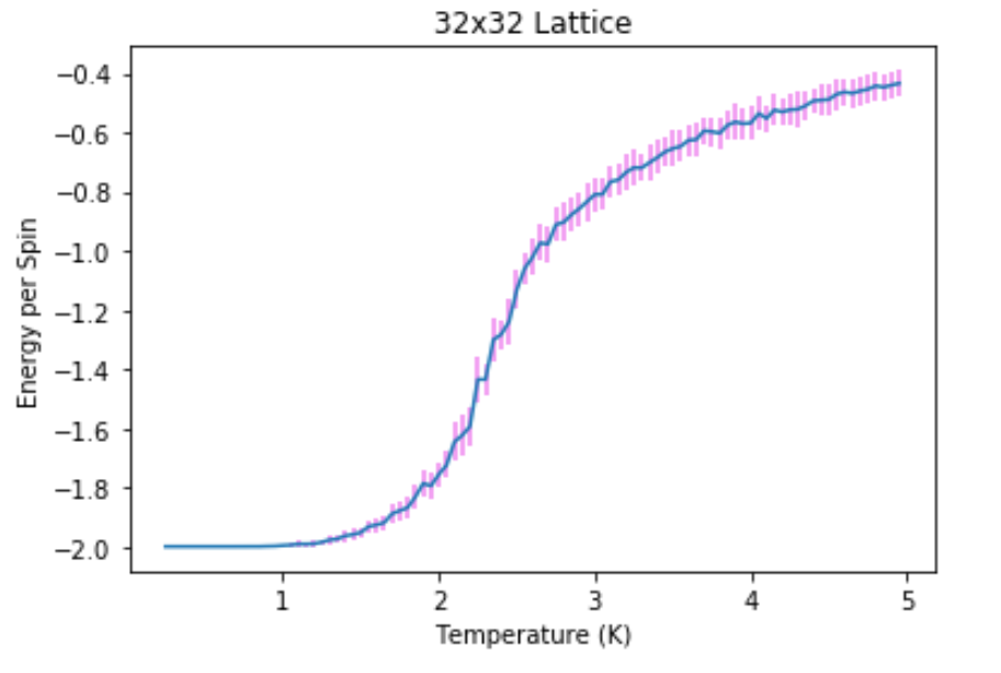
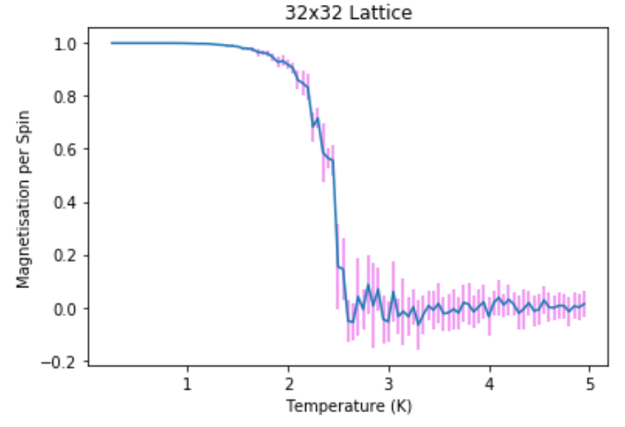
The error bars were produced by calculating the standard deviation.

2x2

4x4

8x8

16x16

32x32

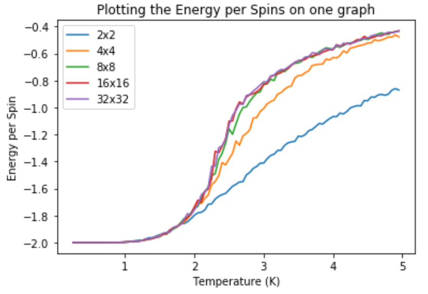
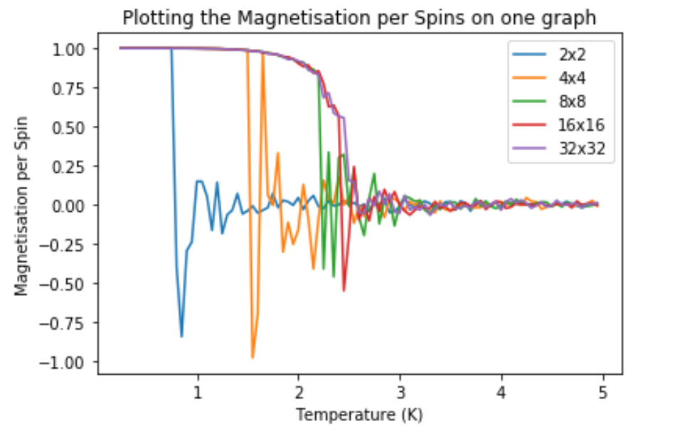
All

The lattice size at which you have long range fluctuations are when the data is less noisy so a lattice size of 16x16 and above.

TASK: By definition, derive

Definition: $C = \frac{\partial ⟨ E ⟩}{\partial T}$

Derivation:

$< E > = \frac{\sum E e x p (- β Δ E)}{Z}$

$< E > = \frac{\partial \ln Z}{\partial β}$

$V a r (E) = < Δ E^{2} > - < Δ E >^{2}$

$V a r (E) = Δ E^{2}$

$V a r (E) = \frac{\partial^{2} \ln Z}{\partial β^{2}}$

$V a r (E) = - \frac{\partial E}{\partial β}$

$C = \frac{\partial ⟨ E ⟩}{\partial T} = \frac{\partial β}{\partial T} \frac{\partial < E >}{\partial β}$

$β = \frac{1}{k T}$

$\frac{\partial β}{\partial T} = \frac{- 1}{k T^{2}}$

$C = \frac{- 1}{k T^{2}} \times - V a r (E)$

$C = \frac{V a r [E]}{k_{B} T^{2}}$

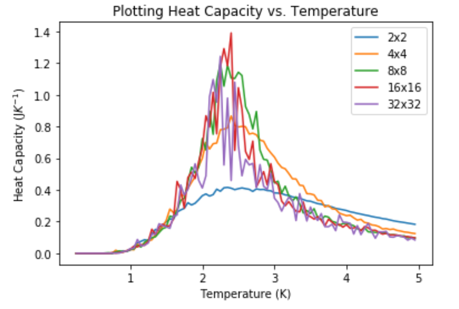
TASK: Write a Python script to make a plot showing the heat capacity versus temperature for each of your lattice sizes from the previous section. You may need to do some research to recall the connection between the variance of a variable, \mathrm{Var}[X], the mean of its square \left\langle X^2\right\rangle, and its squared mean \left\langle X\right\rangle^2. You may find that the data around the peak is very noisy — this is normal, and is a result of being in the critical region. As before, use the plot controls to save your a PNG image of your plot and attach this to the report.

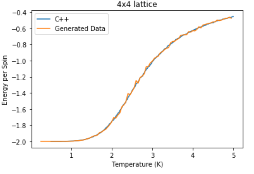
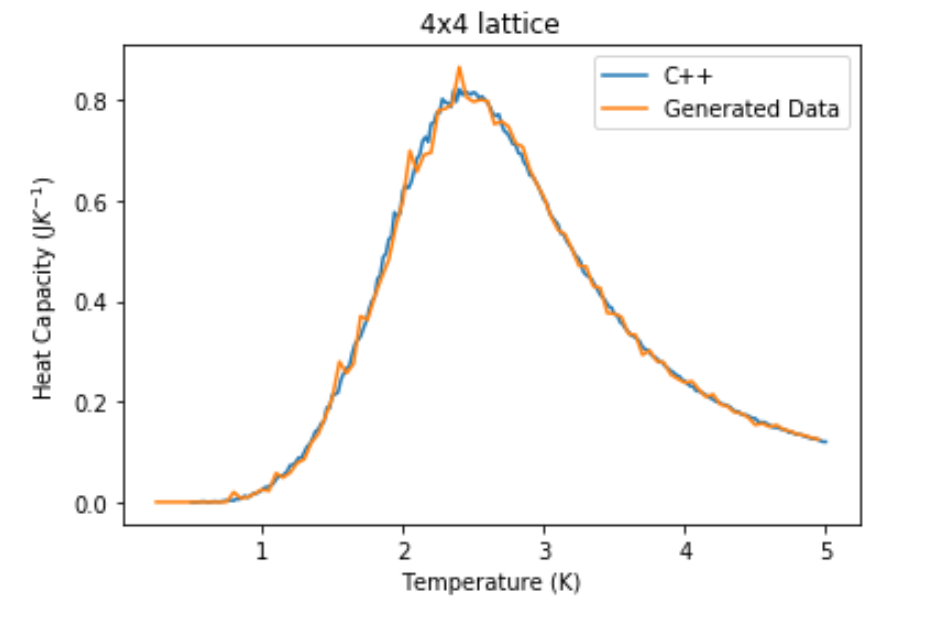
TASK: A C++ program has been used to run some much longer simulations than would be possible on the college computers in Python. You can view its source code here if you are interested. Each file contains six columns: T, E, E^2, M, M^2, C (the final five quantities are per spin), and you can read them with the NumPy loadtxt function as before. For each lattice size, plot the C++ data against your data. For one lattice size, save a PNG of this comparison and add it to your report — add a legend to the graph to label which is which. To do this, you will need to pass the label="..." keyword to the plot function, then call the legend() function of the axis object (documentation here).

The lattice I chose to compare the files with was the 4x4 lattice.

Although they are not perfect, the data I generated tends to fit really well with the C++ generated data.

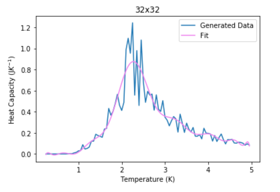
TASK: write a script to read the data from a particular file, and plot C vs T, as well as a fitted polynomial. Try changing the degree of the polynomial to improve the fit — in general, it might be difficult to get a good fit! Attach a PNG of an example fit to your report.

The code used as an example for 2x2ː

              data2=loadtxt('2x2.dat')
              T=data2[:, 0]
              C2=(data2[:,2]-data2[:,1]**2)/(T**2)/4 #calculates the heat capacity from variance and divides by spins
              #first we fit the polynomial to the data
              fit = np.polyfit(T, C2, 9) # fit ninth order polynomial
              #now we generate interpolated values of the fitted polynomial over the range of our function
              T_min = np.min(T)
              T_max = np.max(T)
              T_range = np.linspace(T_min, T_max, 1000) #generate 1000 evenly spaced points between T_min and T_max
              fitted_C_values = np.polyval(fit, T_range) # use the fit object to generate the corresponding values of C

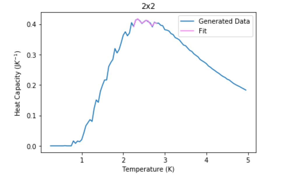
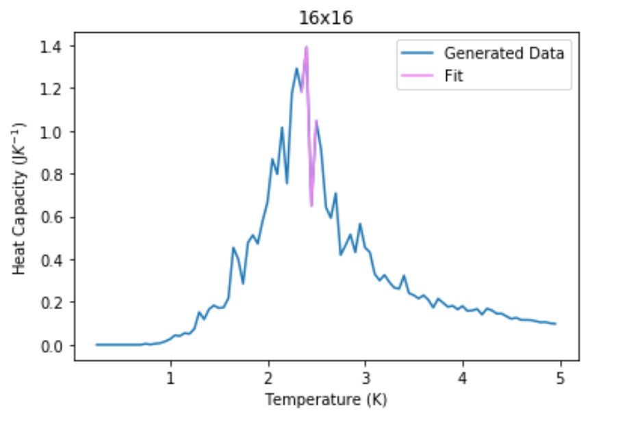
This was difficult because the higher the lattice size the higher polynomials that had to be used to produce non exact fits. So for example bellow 32x32 the polynomial used was 17. You have the peak at the right point but not with the right C value.

TASK: Modify your script from the previous section. You should still plot the whole temperature range, but fit the polynomial only to the peak of the heat capacity! You should find it easier to get a good fit when restricted to this region.

This made it easier to fix the polynomial to a good fit when I just focused on the are which contained the peak- each lattice had a different area and smaller polynomials than for the previous fits. As an example the code used isː

      #now we generate interpolated values of the fitted polynomial over the range of our function
      T_min2 = 2.3
      T_max2 = 2.5

      selection = np.logical_and(T > T_min2, T < T_max2) #choose only those rows where both conditions are true
      peak_T_values = T[selection]
      peak_C_values = C16[selection]

      fit2 = np.polyfit(peak_T_values, peak_C_values, 14) # fit a 14th order polynomial
      fitted_C_values2 = np.polyval(fit2, peak_T_values) #calculate the fit

Different regions were used and the plots are bellow:

TASK: find the temperature at which the maximum in C occurs for each datafile that you were given. Make a text file containing two colums: the lattice side length (2,4,8, etc.), and the temperature at which C is a maximum. This is your estimate of T_C for that side length. Make a plot that uses the scaling relation given above to determine T_{C,\infty}. By doing a little research online, you should be able to find the theoretical exact Curie temperature for the infinite 2D Ising lattice. How does your value compare to this? Are you surprised by how good/bad the agreement is? Attach a PNG of this final graph to your report, and discuss briefly what you think the major sources of error are in your estimate.

The data file I created was:

File:Ks4817MaxCapacity.dat

The code I used was:

     maxcap=loadtxt('MaxCapacity') #loadsdata
     S=maxcap[:,0] 
     Cfin=maxcap[:,1] 
     
     fitcur = np.polyfit(1/S, Cfin, 1) #fits data
     S_rangecur = np.linspace(0, 0.55, 100)
     fitted_C_values = np.polyval(fitcur, S_rangecur) #creates fitted line

The values of C were plotted against 1/Length because it should have a linear relationship so an infinite length would give you 0.

The curie temperature should be 1.4581256797875393 K according to my graph but according to literature it is 2.269. So my value is very much off the real one. Major sources of error would be the one point on my graph which seems to be an outlier but even without that point the value I would obtain would be around 2 not close to the real value so other sources of error could be how I chose to calculate the averages - perhaps I should not have used the same value for all graphs and written a code to estimate when the values were equilibrating or did it for every lattice seperately. It would be interesting to run the stimulations for a wider range of temperatures and lattices but there was not enough time.