Mod:ts tutorial
This is the tutorial page to the 3rd Year TS lab which can be accessed here
Introduction
Within this lab, you will be modelling several chemical reactions and analysing them by calculating Transition State (TS) structures. Locating transition states is an important step in confirming the mechanism of a reaction - for example, is a particular reaction stepwise or concerted? Will certain reaction pathways be favoured? In the lab, you will be analysing the geometry and the MOs of the TS structure and calculating reaction barriers to gain chemical insight into reaction mechanisms.
A simple energy profile (below, left) for a reaction is plotted using the reaction coordinate. Along the reaction coordinate, the TS (2) is the point of maximum energy, linking a set of reactants (1) and products (3). The TS is, therefore, a stationary point (i.e. a gradient of zero) with a negative second derivative along the reaction coordinate.

The energy profile is a 1-dimensional simplification of the full Potential Energy Surface (PES) of the system, where the energy is a function of only one degree of freedom - the reaction coordinate. The system has been set in equilibrium in all other degrees of freedom (minimising) and the degree of freedom relating to the reaction coordinate has been varied. In reality, a chemical system undergoing a reaction will explore more than the reaction coordinate - it can be displaced away from its equilibrium position in any degree of freedom. The potential energy can be plotted against any one or a combination of these degrees of freedom or coordinates. A 2D PES is shown on the right, resulting from varying 2 coordinates. It is an example of the dimerisation of cyclopentadiene. In Coordinate 1 (left to right), the bonding atoms are brought closer together and sp3 hybridised. In Coordinate 2 (bottom to top), the cyclopentadiene molecules are rotated about the reaction centre (twisted). This PES shows some twisting is required to prevent the atoms from getting too close to the highlighted methylene.
These coordinates are in fact the first two normal modes of the system. Recalling the number of normal modes of vibration = 3N - 6, this system with 22 atoms has 60 normal modes. You can have a look at some of the other vibrations in the example above by right-clicking and selecting a model. Models 1-20 are steps of an optimisation calculation, and models 21-80 are the 60 normal modes. You should notice that the first normal mode has a 'negative' frequency. This negative is meant to depict an imaginary number, the result of calculating the frequency of a harmonic oscillator with a negative force constant (square of a negative). At every TS there must be only one imaginary frequency as all other coordinates are minimised.
Gaussian Calculations
To explore the reactions you will need to calculate the reactants, products and TS structures of the system using GaussView and Gaussian.
GaussView can be accessed via the software hub, note that two versions (5 and 6) are available. Both can be used however, the lab is written for GaussView 5 and so some keywords may be slightly different if you use GaussView 6.
From previous labs you should already be familiar with:
- Using GaussView to construct molecules (Make sure you are familiar with the table of controls in the Basic GaussView Tutorial before beginning this tutorial)
- Setting up calculations using GaussView to run with Gaussian
- Running and analysing Optimisation and Frequency calculations for stable minima
- Constructing MO diagrams using ChemDraw
- Viewing and analysing MOs using GaussView
To calculate reactants and products, a suitable starting structure can be drawn in GaussView and then optimised to a minimum using Gaussian. When you are optimising to a minimum all degrees of freedom are altered to try to minimise the energy. The resulting minima will be your stable reactants/products. You can use a frequency calculation to confirm that you are at a minimum energy structure by checking that all of the normal modes are real (positive in Gaussian).
Transition State Calculation
The calculation of TS structures is less straightforward. The TS is a maximum in one degree of freedom (the reaction coordinate) meaning that a conventional optimisation (where all degrees of freedom are minimised) doesn’t work. Instead, a different method - a TS Optimisation - is used in Gaussian. This method requires at least one imaginary (negative in Gaussian) frequency which the TS optimisation can follow.
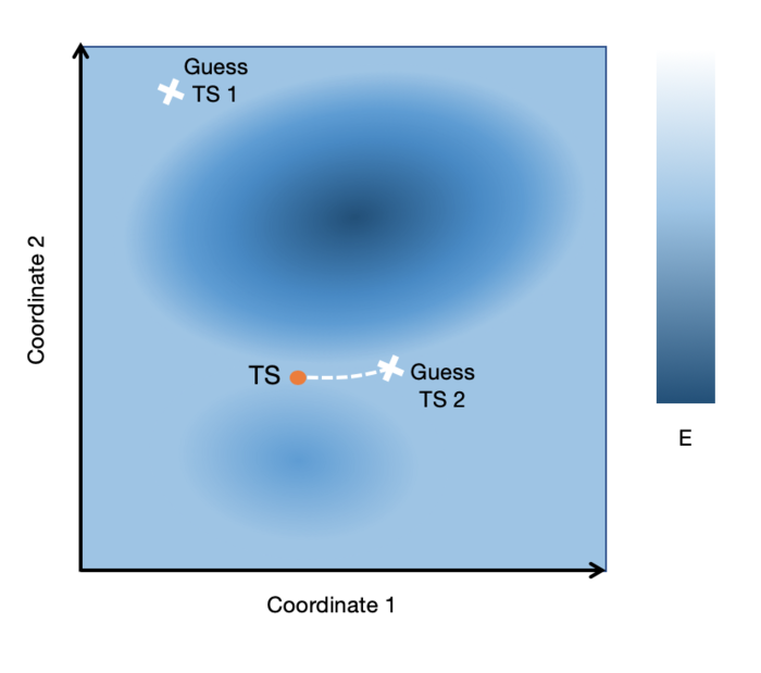
When starting a TS Optimisation, it is important to begin from a guess structure which is close to the first-order saddle point structure that you wish to locate. The worse the starting guess structure is, the more likely that the calculation will fail to find the correct TS. For example, in the image below, the guess TS 1 structure is too far away from the actual saddle point. The calculation would struggle to find the correct TS structure and will most likely fail. In most cases, the wrong TS will be found (check the negative vibrational mode - does it look like the motion you would expect to see?) or there will be multiple imaginary frequencies. A converged structure with multiple imaginary frequencies is indicative of a higher-order saddle point. In comparison, guess TS 2 is much closer to the structure it is aiming to find and will be more likely to locate the TS successfully.
Chemical intuition plays a large part in starting from a suitable guess TS structure. Below is the general procedure for setting up and submitting Gaussian TS Optimisations. The tutorial exercises will take you through approaches for generating the TS structure to use in step 1.
1. Generate a guess TS structure Use one of the approaches described in the tutorial exercises to generate your guess TS structure. 2. Calculation set up In the Job Type tab:
In the Method tab select the method to use:
In the Additional Keywords box at the bottom, type: opt=noeigen. Press 'Submit' and follow the prompts to save the input file with an appropriate name. The calcualtion should then run, these can take some time (depending on the size of the molecule and the method being used). Only one can be run at a time, wait for it to finish or if it seems to be taking a very long time (hours!) then seek help. 3. Analysing the calculation If the job succeeds, open the log file. If it doesn't, contact a demonstrator or go to the Troubleshooting page. Hopefully, the final structure should look like the TS you were expecting. To analyse the structure:
If there is more than one negative frequency then you have a higher order saddle point, if there are no negative frequencies then you have a minimum energy structure. This is likely to be because the starting structure input to the calculation was not close enough to the real TS structure on the PES. Reopen your input file and try to ammend the structure to make it closer to what the TS will resemble. Also try checking the Troubleshooting page or contact one of the demonstrators. If the structure has a single imaginary frequency then it is a TS. Check that it is the correct TS by choosing it and pressing 'Start Animation'. The vibration should correspond to the reaction coordinate (i.e. it should look like it's going between the reactants and products).
4. Reoptimise with a more accurate method If the results are fine and you used PM6 then you can now reoptimise with a more accurate method if necessary. Copy the structure to a new window (Shortcut: ctrl + (C, N, V) ). Changing the method, repeat step 2 and 3. |
Tutorial Exercises: Generating a guess TS
Approach 1: Straight Guess
The first way to locate a TS is to just draw a guess structure and run a straight TS Optimisation on this. This usually fails and is not recommended unless you are very sure that you are close to the TS and have a very small system.
Advantages: Fastest method
Disadvantages: Very unreliable. Requires knowledge of the TS
1. Draw a guess TS structure using GaussView. This can be from previously optimised fragments (with copy-and-paste). In bond-forming reactions, the distances between the reacting atoms will be somewhere in between the reactant and product distances. For example, the C-C distance in the TS of a C-C forming reaction will be somewhere in between their combined Van der Waals radii and a C-C bond length. The value of 2.2 is often used for C-C bond forming reactions. 2. Set up and run the TS Opt calculation by the procedure above |
Practice: Cope Rearrangement
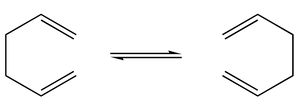
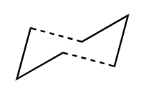
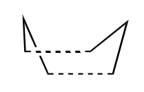
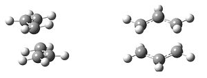
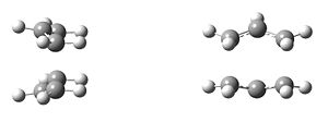
The classic example of a Cope rearrangement is the [3,3]-sigmatropic rearrangement of 1,5-hexadiene. Its mechanism has been debated for a long time (stepwise/dissociative/concerted) but it is now accepted that it rearranges in a concerted, pericyclic fashion via a diradical transition state. This TS bears similarity to either the cyclohexane boat or chair conformation:
|
| |
|
| |
| Chair Transition State | Boat Transition State |
|
Approach 2: Freezing Atoms
This method requires drawing a guess TS structure and freezing the atoms directly involved in the reaction. Optimising the structure to a minimum allows the rest of the degrees of freedom, which are not involved in the reaction mechanism, to equilibrate while the frozen atoms are prevented from moving. This ensures the system is as close as possible to the TS before the actual TS optimisation.
Advantages: Fastest reliable method
Disadvantages: Requires knowledge of the TS
1. Follow approach 1 by drawing a guess TS structure. Make sure the distances between the atoms that you will freeze are reasonable. 2. Freeze the distances between the atoms involved in the reaction (note that GaussView and Gaussian refer to these distances as 'bonds' even though they might not be 'bonded'). To do this, click on 'Edit' then Redundant Coordinate Editor. On the molecular editor window, select the atoms of a bond to freeze. Go back to the Redundant Coordinate Editor and change 'Unidentified' to 'Bond', 'Add' to 'Freeze'. For each atom pair, you need to add a coordinate. Before closing the window, make sure there are no errors (shown at the bottom of the window) and that the correct pairs are frozen. 3. Set up the calculation. You should notice that the keywords line now contains opt=modredundant. 4. When the job has terminated successfully, open the log file in GaussView. Check that the frozen 'bonds' have remained the same length. Now copy this geometry into a new window and run a TS optimisation on the structure. Ensure that frozen bonds are removed in the TS calculation. Gaussian will behave unpredictably if you attempt to search for a TS with bonds still frozen. |
Practice: Cyclopentadiene Dimerisation
If you've used cyclopentadiene in the lab, chances are you've needed to 'crack' it. The reason for this is that cyclopentadiene dimerises with a half-life of hours at room temperature, or more slowly at lower temperatures. This dimerisation is an example of a Diels Alder reaction. Cracking is the process of heating it to reverse the reaction back to the reactive monomer. This is due to the negative entropy of the reaction that disfavours dissociation, which becomes more significant at higher temperatures.
Repeat the above for the exo TS. Minimise the reactants for both the endo and exo and compare the reaction barriers. Which is more kinetically favourable? Now minimise the products and compare the reaction energies. Which is the more thermodynamically favourable? |
Approach 3: Starting from Reactants/Products
Sometimes we will not know enough about the form of the TS to draw a guess structure straight away. In this case, we can start from either the reactants and products, changing bond lengths to resemble the TS.
Advantages: More reliable than previous methods. Doesn't require much knowledge of the TS.
Disadvantages: Requires additional steps. Difficult if minima are far away in geometry from TS. There can be problems if you start from the products but your TS resembles the minima.
1. At this point, you'll need to decide whether to use the reactants or the products. As a general rule, choose whichever has the fewest molecules, so for a dimerisation reaction choose the dimer. Draw and optimise this structure. Open the resulting log file and check it's the correct structure. Copy this structure into a new window. 2. Decide which lengths and/or angles will change during the reaction. Modify them using the appropriate editing tools. Often it's enough to just change the atoms directly involved in the reaction, but if this doesn't work, try altering neighbouring atoms to reflect the change in hybridisation they might undergo. In a classic Diels Alder reaction, for example, 3 double bonds become single bonds and one single bond becomes a double bond, so it might be worth changing these values to somewhere in between. The dienophile carbon atoms become sp3 hybridised, so the neighbouring atoms might need to be distorted a little to reflect this. 3. Follow approach 2: freeze the degrees of freedom you think are involved in the reaction coordinate and optimise, then run a TS optimisation on the resulting (unfrozen!) structure. |
Practice: Xylylene-SO2 Diels Alder Cycloaddition
This is an example of a hetero-Diels Alder reaction, where SO2 is used as a dienophile. Without knowing the direction of approach of the SO2 or whether the barrier is early or late, it can be difficult to use draw a guess TS directly. Therefore, we'll start from the product.
Aside from endo/exo conformers, there is an entirely different way for SO2 and xylylene to react known a cheletropic or chelotropic reaction. Try using the above to find the TS for a cheletropic reaction between the sulfur of SO2 and xylylene. This time, start with an iso-indene fragment. Compare the reaction barriers and enthalpies of reaction between the two reactions. |
Appendix
Analysing Calculations
Convergence
Check that the job has properly converged. For each step in optimisation, the gradient will be calculated to determine if the system is at a stationary point. To prove that a stationary point has been found, open the log file and scroll from the bottom to find a section that looks like this:
         Item               Value     Threshold  Converged?
 Maximum Force            0.000098     0.000450     YES
 RMS     Force            0.000010     0.000300     YES
 Maximum Displacement     0.001379     0.001800     YES
 RMS     Displacement     0.000379     0.001200     YES
 Predicted change in Energy=-4.942954D-08
 Optimization completed.
    -- Stationary point found.
This job has landed on a stationary point. Compare to the following, which did not converge properly:
         Item               Value     Threshold  Converged?
 Maximum Force            0.000155     0.000450     YES
 RMS     Force            0.000021     0.000300     YES
 Maximum Displacement     0.002340     0.001800     NO
 RMS     Displacement     0.000561     0.001200     YES
 Predicted change in Energy=-2.681147D-07
Frequency Calculation
If you haven't already done so, run a frequency calculation on the job (remember to hold parameters the same - method, basis set, solvation etc).
For a reactant or product then check that all of the vibrations are positive. For a TS, check that you have one negative vibration and that it corresponds to the reaction by visualising the vibration (Results, Display Vibrations). This is a very good indication that you have the correct TS structure.
Intrinsic Reaction Coordinate (IRC) Calculation
Once you have your TS, you can run an IRC to confirm that it is the correct structure. An IRC follows the minimum energy pathway to reactants and/or products on the PES. By checking the end structures given by the IRC to the products/reactants that you expect to form then you can confirm that the TS links the correct two minima.
1. Calculation set up Using your optimised TS structure set up a Gaussian calculation. (Note: Your starting structure must have only one imaginary frequency to run an IRC) In the Job Type tab:
2. Check calculation IRCs can be problematic, especially for reactions where the PES is not well defined. Some common problems with IRCs are shown below and if you are having trouble getting them to run successfully ask a demonstrator. Otherwise, if the IRC has run until a stationary point has been found in both the reverse and forward direction then you can analyse the endpoints to confirm the TS. 3. Confirming the TS Take the first and the last step of the IRC. (I.e. the endpoints of both the reverse and the forward pathways). Optimise the structures to a minimum. Once complete open the log file in GaussView - do the optimised structures look like the products/reactants you expect? Compare them to your optimised reactants and products - are they the same? If so then your TS links the correct two minima on the PES. For a unimolecular reaction then optimising the endpoint structures will work well. When there are two or more reactants, an optimisation becomes very difficult as the PES is bumpy and the gradients are small. This can yield reactants/products in the IRC that are irrelevant to the reaction - don't use these for your reaction profiles. |
Reaction Barriers and Reaction Energies
Barriers and reaction energies can be calculated at room temperature and 0K using information from the log file of a frequency calculation. You will need to run a frequency calculation for each of the optimised reactants, TS and products. Using Notepad or Notepad++, open each log file and search for a section named "Thermochemistry".
For 0K, the value to use is the "Sum of electronic and zero-point Energies".
For room temperature, the value to use is the "Sum of electronic and thermal Free Energies".
If there are multiple reactants/products then make sure that you use the optimised isolated structures (the assumption that they react from infinite separation) to calculate the correct energy barrier from.
Useful Tips and information
Comparing results of jobs
When comparing energies between structures, it's important to ensure that the energies are calculated in the same way. In every case, make sure the computational method, basis set, solvation method, convergence criteria and grid are the same. This means if you are using "int=grid=ultrafine" or "opt=tight" in one calculation, it must be used in all calculations for structures that are being compared.
Bond types are ignored by Gaussian
In a quantum mechanical calculation, all Gaussian uses from the geometry is the distances between the atoms. This means specifying a bond type is meaningless and mostly aesthetic - it won't remove two hydrogens if you change a single bond to a double bond. However, they are very important in a molecular mechanical calculation! Check that the number of atoms is correct in all calculations.
Job Monitoring
For jobs that are expected to take a long time or are taking longer than expected, it's worth opening them in GaussView to see how they are doing. In GaussView, choose File then Open. Locate the log file of the job you want to monitor and make sure 'Read Intermediate Geometries is selected and open the file. Now you can periodically refresh the job with File, Refresh. Check that the job looks like it's converging to the correct geometry.
Creating a follow-up job manually
If a checkpoint file (.chk) exists for a file, Gaussian can read the output of it as the input of a new calculation. This has numerous advantages:
- A step in generating the guess wavefunction can be skipped (it's taken from the previous job)
- Force constants can be read into calculations such as IRCs
- Easier to be consistent between calculations
- Additional features, such as restarting previously failed calculations
The drawback is that it's much harder to get used to than GaussView. The general structure of a follow-up input file is:
%mem=<memory>
%nprocshared=<processors>
%oldchk=<old checkpoint path>
%chk=<new checkpoint path>
# <keywords> guess=read geom=allcheck
<NEWLINE>
Note that all Gaussian inputs must finish with a new line - the parser will read sections until it encounters a newline character, and finish if it reaches the end of a file.
Create the file using Notepad ++. For the memory, choose 1GB to begin with. You might need more if the program runs out of memory. For processors, choose the number of physical processors that you want to run on, which will be up to 4 for the Windows computers. Direct %oldchk to the path of the checkpoint file you want to read from. Note that it should be an absolute path. Input the keywords as required. Save the file with the extension '.gjf'. In an Explorer window, drag the file into an instance of G09 and click Run.
Restarting failed jobs
Sometimes optimisations or IRC calculations fail for a variety of reasons. Create a follow-up input file. If you need to restart an optimisation, add into the keywords opt=restart, or for an IRC, add IRC=restart. Note that if the keywords opt or IRC already exist, you'll need to add restart into the existing keywords.
Troubleshooting
If you encounter errors or problems with any part of this lab, feel free to discuss them with any of the demonstrators. If a demonstrator isn't around, see this link for Gaussian troubleshooting.
IRC Troubleshooting
Gaussian will often produce an IRC that seems reversed. This is normal and is the result of not providing information as to what the reactants and products are. It can be corrected by identifying a bond that will lengthen over the course of the reaction, for example a bond breaking, or a double bond becoming a single bond. Once the two atoms (N1 and N2) are identified, include this line in the IRC calculation replacing N1 and N2 with the atom numbers:
irc=(phase=(N1,N2))
| Example IRC | Notes/Solutions for errors |
|---|---|
|
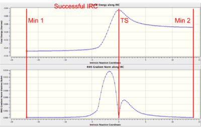
A successful, asymmetric IRC.
Note that the gradient must be 0 at the TS, reactants and products (minima). |

|
Failed IRC as the initial geometry is not a TS.
This can happen when the method and/or basis sets are not consistent between the TS and IRC calculation. |
|
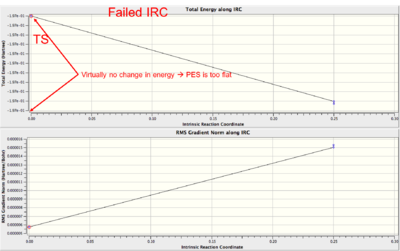
Failed IRC as the PES is too flat at the TS and the algorithm cannot decide which direction to move down.
See this page for a fix. |

|
Failed IRC at the first or last point on the IRC. The gradient is 0 here, but it fails as it is not a minimum.
See this page for a fix. |
