Mod:scan

Submitting calculations to the Departmental HPC Cluster

The Chemistry department has access to a HPC (high performance computing) system which can be used to run more time consuming calculations than is possible interactively on a single computer whilst sitting in front of it.

One far more reliable and quantitative way of modelling a molecule is to subject it to quantum mechanical modelling using Density Functional theory. In practice, this is implemented here using a program called Gaussian 09. The procedure to submit such a job is as follows:

Creating an Input file

After you have optimised your sketched molecule using Avogadro or Gaussview, as described previously, you will have a Gaussian input file saved in your H: drive by default.
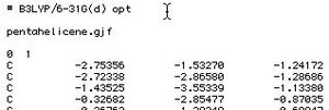
Typical Gaussian input
The file will have to be edited before it can be submitted. You can do this either with Gaussview as the program, but a much simpler method is to open the file (pentahelicene.gjf in this example) using eg the Windows Notepad++ editor. Remove any existing lines starting with % or # and replace them with one of the following single lines (the second example also results in the vibrational frequences and from these the entropy being computed, and hence the zero-point and free-energy corrected value, ΔG). This latter option will take significantly longer however.

# B3LYP/6-31G(d) opt
or
# B3LYP/6-31G(d) opt freq
to produce a file that looks like the one shown on the right.

For a molecule the size of e.g. pentahelicene, the calculation will take about 4-5 hours overnight. If for some reason, your molecule is taking longer, you can always reduce the size of the basis set to e.g. B3LYP/3-21G*, or submit the job on a Friday, when it will have the entire weekend available to it. If you want greater accuracy (but for longer computing time), try e.g. # B3LYP/cc-pVTZ opt freq.

Submitting the Input file

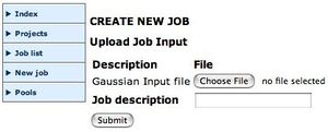
Create a new job
You will have to login as yourself. You can submit as many jobs as you wish through this mechanism, but you must prepare an input file for each first (.gjf if you want to run Gaussian).
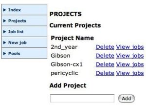
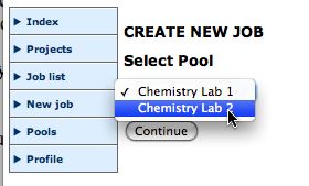
Create a project
Select a pool
After you are logged in you should organise your jobs by project. Create a suitable new project, then select New job.
1. Compchem Lab 1 runs continuously during the day and night, has a concurrency of 8 and a time limit of 48 hours.
Next, select an Application. Two types of Gaussian can be selected: Gaussian 4px and Gaussian 8px
Next select the Project you have just created, and press Continue.
Upload your input file
You now have to find the Gaussian input file, as prepared above. You should Browse to drive H: to find this file. Add a description which will help you identify the job.
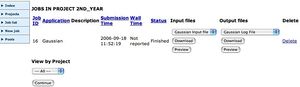
The Chemistry Condor Pool
The job will be added to your list of jobs, and you can view its status, which is either running if there is a vacant slot in the queue you submitted to, or pending if there is not. Unfortunately, you cannot find out how many jobs are in front of yours for a pending job. If a module deadline is approaching, everyone will be submitting jobs, so it is very much in your interest to submit jobs early rather than at the last possible moment! Be aware that the time taken to run a Gaussian job depends critically on the size of the molecule, it scaling at around N⁴, where N is the number of (non-hydrogen) atoms. Typically, a molecule with around 12 (non-H) atoms will take around 30 minutes, but one with 24 would take around eight hours (or more depending on how floppy it is, and what kind of basis set you have requested). Calculations of optical rotations also take a long time.
Viewing the outputs
When the job has completed, click on the Job List link. This will show all available outputs. Download the program Log file (this will help you chart whether the calculation was successfull) or the Gaussian Formatted Checkpoint file onto the desktop of the computer you are using. Double-click the file which should open up Gaussview, where the molecule can be viewed and checked. You can use the latter file to e.g. plot molecular orbitals for the molecule, view vibrational modes, etc. Full details of these procedures are described in the Gaussview and Gaussian manuals.

Archiving the output into a digital repository

Depositing an entry in DSpace

A very recent innovation is the Institutional digital repository, a resource for permanently archiving calculations, spectra and crystal structures. You can get a flavour of this by archiving your own calculation in the SPECTRa digital repository. To the right of the Portal display is a link termed Publish. If you click on this, and the calculation is actually in a state to be published (it may for example have failed for some reason) then appropriate metadata for the calculation is collected, and the collection deposited into the repository. From here, it can be retrieved in future, and it can also be cited in the manner of a DOI, i.e. http://dx.doi.org/10042/to-ABCD where ABCD are the four integers representing your deposition ID. In a Wiki, cite this in the form of DOI:10042/to-2253

A Note on Publishing to D-Space

In order to publish to an archive, you must first select the archive you want to publish to:

1. Log in to the HPC

2. Click on "Profile" in the bottom left

3. Tick the "Publish to DSpace" box

4. Click "Update"

When you click "Publish" in your job list, your files will now publish to the archive you have chosen.

Retaining the Calculations

Do not delete any completed jobs from the submission pages until your report has been graded. You may be asked to show individual jobs (via the input, or outputs) if for example the calculation has not succeeded in the manner you expected and you would like feed back on this or any other errors.