Mod:Hunt Research Group/z-matrix
Optimisations, partial optimisations, scans and the z-matrix
optimisations and errors
- can be carried out in a range of coordinates, the most common are internal coordinates (bonds, angles, torsions)
- cartesian coordinate and z-matrix can also be used, these are more advanced options
structure is oscillating
- and not converging or converging very slowly
- is your structure really converged and just cannot quite reach the convergence criteria, check the ITEM section
- try optimising with cartesian coordinates OPT=(cartesian)
- do a frequency analysis are they all positive!
- if not then use the computed force constants to restart the job OPT=readfc geom=checkpoint guess=read on a restart
slow convergence when performing a scan
- trouble with very long runs with only a small change OPT=(maxcycles=15)
- this will of course force the scan to move on from a not completely optimised geometry
- you may need to go back and complete the optimisation
failed optimisation
- did it have enough steps? Just restart it using the checkpoint file geom=checkpoint guess=read
in a scan there are coordinate issues
- trouble converging? Is there an error related to a bond angle going to 180º
- then you need to break the symmetry of the angle, or less often redefine the angle another way
- try optimising with cartesian coordinates OPT=(cartesian)
- a curvilinear step failure?
 Add virtual bond connecting atoms H3         and B1         Dist= 2.87D+00.
 The following ModRedundant input section has been read:
 B       2       3 1.5000 B
 B       2       3 S   4 0.1500

 Iteration  1 RMS(Cart)=  0.00662620 RMS(Int)=  0.00675248
 New curvilinear step failed, DQL= 7.94D-02 SP=-4.68D-04.
 RedCar failed in NewRed.
 Error termination via Lnk1e in /apps/gaussian/g09_d01/g09/l101.exe
- look at the section just before the failure, has gaussian tried to add a new coordinate that is linear!
- this is the case in the job above
- we need to manually remove the coordinate and angle
- for example see below where we have removed the offending added bond between H36 and B1 as well as the angle
B 36 1 R
A 35 36 1 R
partial optimisations
- involve freezing one coordinate while allowing all others to optimise
- very occasionally you freeze more than one coordinate, but the errors introduced become larger the more coordinates you freeze
- use OPT=(modredundant)
- in addition you add a section after the coordinates and connectivity
- identify the coordinate type B(bond), A(angle),T(torsion)
- give the atoms defining the coordinate and the value you want them to have
- give the atoms defining the coordinate and F to freeze the value
- if you want to activate the coordinate later change the F to A (activate)
- the following example is for two water molecules
- we define a bond between atoms 1 and 3 (O and H) to be 1 angsrom
- then we ask for this bond to be frozen
- in most cases there is a single important coordinate, but you can add more coordinates after the one given
%mem=1GB
%chk=2water.chk
# opt=(modredundant,maxcycles=12) b3lyp/6-31g geom=connectivity

Two water molecules

0 1
 O                 -1.26602562   -0.36057693    0.00000000
 H                 -0.30602562   -0.36057693    0.00000000
 H                 -1.58648021    0.54435890    0.00000000
 O                 -1.97115382    2.44391033    0.00000000
 H                 -1.01115382    2.44391033    0.00000000
 H                 -2.29160840    3.34884617    0.00000000

 1 2 1.0 3 1.0
 2
 3
 4 5 1.0 6 1.0
 5
 6

B 1 3 1.0
B 1 3 F
relaxed scan
- involve specifying the value of one key coordinate and optimising all others
- the key coordinate is then varied in a systematic way
- use the OPT=(modredundant) keyword
- then in the section after the coordinates and connectivity add
- identify the coordinate type B(bond), A(angle),T(torsion)
- give the atoms defining the coordinate and the value you want them to have
- specify you want a scan with S and then the number of steps and the change in the variable on each step
- the following shows how you change the modredundant part of the input file
- here the O-H bond is specified and set to 1 angstrom
- then identify the coordinate and specify a scan (S) this time we will take 5 steps of 0.15
- this will carry out a partial optimisation for the r(O-H) coordinate set to the values =1.0,1.15,1.30,1.45 and 1.60
B 1 3 1.0
B 1 3 S 5 0.15
simple scan
- involve specifying the value of one key coordinate to alter on each step, all other coordinates are frozen
- this can be used to get a rough idea, it is not advisable to use this option
- use the SCAN keyword
- the molecular structure must be entered as a Z-matrix, more on the Z-matrix below
complex partial optimisations
- there are times when you want to freeze one coordinate and then scan another
- for example in H-bonds X---H---Y, you want to freeze the "bond" or distance between X and Y and then scan the H moving between them
- some of the options identified in the manual DO NOT WORK
- to freeze two atoms, use -1 in the cartesian coordinates (those not specified default to optimisation)
- add the redundant coordinate as usual
- the following freezes the oxygen atoms in place and then scans the O-H distance
%mem=1GB
%chk=test.chk
# opt=(modredundant) b3lyp/6-31g geom=connectivity

Title Card Required

0 1
 O  -1             -1.26602562   -0.36057693    0.00000000
 H                 -0.30602562   -0.36057693    0.00000000
 H                 -1.58648021    0.54435890    0.00000000
 O  -1             -1.97115382    2.44391033    0.00000000
 H                 -1.01115382    2.44391033    0.00000000
 H                 -2.29160840    3.34884617    0.00000000

 1 2 1.0 3 1.0
 2
 3
 4 5 1.0 6 1.0
 5
 6

B 1 3 1.0
B 1 3 S 5 0.15
- the output will look something like this
Initialization pass.
                           ----------------------------
                           !    Initial Parameters    !
                           ! (Angstroms and Degrees)  !
 --------------------------                            --------------------------
 ! Name  Definition              Value          Derivative Info.                !
 --------------------------------------------------------------------------------
 ! X1    R(1,-1)                -1.266          Frozen                          !
 ! Y1    R(1,-2)                -0.3606         Frozen                          !
 ! Z1    R(1,-3)                 0.0            Frozen                          !
 ! X4    R(4,-1)                -1.9712         Frozen                          !
 ! Y4    R(4,-2)                 2.4439         Frozen                          !
 ! Z4    R(4,-3)                 0.0            Frozen                          !
 ! R1    R(1,2)                  0.9653         estimate D2E/DX2                !
 ! R2    R(1,3)                  1.0            Scan                            !
 ! R3    R(3,4)                  1.8987         estimate D2E/DX2                !
 ! R4    R(3,5)                  1.9826         estimate D2E/DX2                !
 ! R5    R(4,5)                  0.9554         estimate D2E/DX2                !
 ! R6    R(4,6)                  0.9807         estimate D2E/DX2
The Z-Matrix and optimising linear bonds
The z-matrix is an additional method of describing atomic positions. This is very well described on the Gaussian webpage. | Gaussian Z-matricies
Using Gaussview to build a z-matrix is generally a bad idea. While I was working with simple molecules it completely failed to build a z-matrix, instead building some weird cross over between cartesian coordinated and z-matricies that didn't make any sense. It is best to construct the z-matricies manually (if dealing with small molecules) using Gaussview to give bond lengths and angles.
Using a Z-Matrix to build a pentagon
A
B  1  1.5
C  2  1.5    1  108
D  3  1.5    2  108    1  0.0    0
E  4  1.5    3  108    2  0.0    0
The 0 at the end of lines 4&5 in the Z-matrix indicate that the final value is a dihedral angle. If this was to be a 1, the final value would be a second angle.
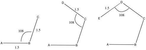
It doesn't matter where atom A is, as it is being used a reference point. Atom B is connected to atom A (indicated by the 1) at a distance of 1.5. Atom C is connected to atom B (indicated by the 2) at a distance of 1.5, with an A-B-C angle of 108. Atom D is connected to atom C at a distance of 1.5, with a B-C-D angle of 108 and a dihedral angle of 0.0 Atom E is connected to atom D at a distance of 1.5, with a C-D-E angle of 108 and a dihedral angle of 0.0
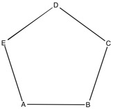
The building of a pentagon is shown below.
It is possible to include variables that occur throughout a molecule, for example the C-H bond lengths in a long alkyl chain. This is done by using a term within the main body of the input, and the second line beneath the z-matrix putting the term and the value for the bond length/angle. As the N-H bonds lengths and angles will all be the same in the input structure the z-matrix has become.
A
B  1  B1
C  2  B1    1  A1
D  3  B1    2  A1    1  0.0    0
E  4  B1    3  A1    2  0.0    0

B1  1.5
A1  108
The term B1 refers to the N-H bond distance, the A1 term refers to the H-N-H bond angle
It is also possible to include values which you wish to keep constant. This is done in a similar way to including variables. To include constants a empty line should be left after the variables, and then the constants are written, again using a term found in the z-matrix. To fix the bond length, the next z-matrix is needed.
A
B  1  B1
C  2  B1    1  A1
D  3  B1    2  A1    1  0.0    0
E  4  B1    3  A1    2  0.0    0

A1  108

B1  1.5
If working with a larger molecule it is worth looking into combining z-matricies with cartesian coordinates, again this is explained well on the Gaussian webpage. Each atom can be described using either cartesian coordinates or z-matrix. If a atom is being described using a z-matrix the atoms used to define its position need to be included above the z-matrix line, using either a z-matirx or a cartesian coordinate system.
Y  0       -0.10608500   -0.05799800    0.01993400
Cl 0       -1.25351400   -1.98304000    1.34042900
Cl 0        1.62975500    1.12134800    1.60905800
Cl 0        1.11223600   -1.09533800   -1.98836000
Cl 0       -1.76438600    1.62418700   -0.79499400
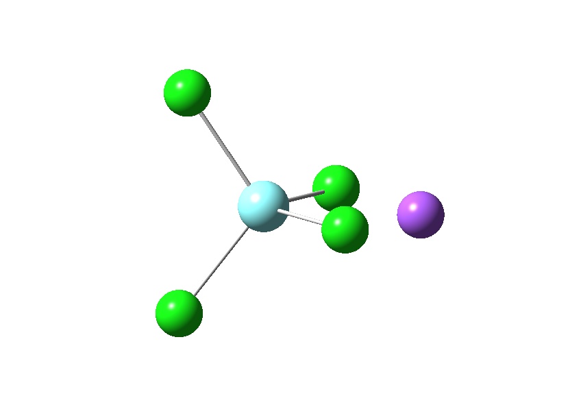
Na        4 2.556   1 71.370  5 -1.410 0
An example showing how an atom which is not bonded to the complex can be represented via a different method for describing atomic positions.
Optimising Linear bond
To optimise linear bonds a dummy atom needs to be introduced. On the gaussian webpage linked earlier there is a section on how to introduce dummy atoms into calculations.
Dummy Atoms
Although being used here to help optimise linear bonds, the dummy atom is useful for other tasks, such as the optimisation of the NH3 molecule. Using a dummy atom allows for the angle between the lone pair and the H atoms to be more effectively described and retain the C3V structure.
N
X 1 1.
H 1 nh 2 hnx
H 1 nh 2 hnx 3  120.0
H 1 nh 2 hnx 3 -120.0

nh 1.0
hnx 70.0
So here the nh bond length is set to 1.0 and the hnx bond angle is set to 70.
When introducing dummy atoms to linear bonds it is essential that the dummy atom is 'bonded' to the central atom, allowing the atoms either side to be set from the dummy atom. 'Bonded' is in quotes as the dummy atom should never have a formal bond attaching it to anything, think of it more as a point in space relative to the central atom of the linear bond.
Although optimising the CO2 molecule doesn't appear to need a dummy atom to be optimised, it has been included here to show one way of introducing it.
C
O   1  1.2
O   1  1.2   2 180.0
X   1  1.0   2 90.0   3 90.0 1
The 1 at the end of the X input line represents a second angle needed for defining the linear angle. A dihedral can be used but its slightly more complex.


