Mod:Hunt Research Group/electrostatic potentials
Visualizing Electrostatic Potentials
Generating the Surface
1. Log yourself in to the IC high-performance computer.
2. Load the Gaussian module in your terminal using the keyword: eg. module load gaussian/g03-e01
3. Take the checkpoint file of the molecule to be examined and convert it into a formatted checkpoint file using the formchk utility (eg. formchk water.chk water.fchk).
4. The formatted checkpoint file can then be used to generate various cubes (surfaces), such as molecular orbitals, the total electron density and electrostatic potentials using the keyword cubegen.
5. Electrostatic potentials requires that first the total electron density is generated. The default command to do this is: cubegen 0 density=scf name.fchk name.cube 0 h. For example, for water you would type cubegen 0 density=scf water.fchk water.cube 0 h. Now wait until your usual prompt returns.
6. You are now able to generate the electrostatic potential surface. You use the same default command as for the total density but changing the word density to potential. You must also change the name of the cube file that is to be created so that it does not overwrite the cube file for the total electron density. For example, for water you would type cubegen 0 potential=scf water.fchk water_ESP.cube 0 h. Wait again for your prompt to return (this may take a little longer, particularly if the molecule is large).
7. Now copy (keyword: scp) the formatted checkpoint file and two cube files from the hpc to your computer's hard-drive and open the formatted checkpoint file with Gaussview.
8. Click on the Results tab and then Surfaces/Contours.
9. Click on Cube Actions and then Load Cube from the drop-down menu; select your total electron density cube file (water.cube in this case). The words 'Electron density from Total SCF Density (npts...)' should appear in the Cubes Available box.
10. Click on Surface Actions and then New Surface from the drop-down menu. The words 'Electron density from Total SCF Density (isoval = 0.0004) (Showing)' should appear in the Surfaces Available box. The surface (total electron density) should also now be being visualized over your molecule (it may take a few seconds to generate the mesh). In the case of water it should appear as follows:

11. Now to visualise the electrostatic potential, click again on Cube Actions and then Load Cube from the drop-down menu and select you electrostatic potential cube file (water_ESP.cube in this case). The words 'Electrostatic potential from Total SCF Density (npts...)' should appear in the Cubes Available box.
12. In order to visualise the electrostatic potential properly, you must first hide the total electron density surface presently on your molecule. This can be done by selecting Hide Surface from the Surface Actions drop-down menu. It should disappear.
13. Now click on Surface Actions again and then New Mapped Surface from the drop-down menu. A small box should appear: select Use an existing cube and then Ok. The words 'Electron potential from Total SCF Density (isoval = 0.0004 ; [mapped...]) (Showing)' will appear in the Surfaces Available box.
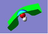
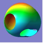
14. When you examine the surface, you should notice that it appears very strange. For example, in the case of water it appears as follows:

15. This is because if you look in the Cubes Available box, you will notice that the Electrostatic Potential from Total SCF Density is highlighted. However, it is the Electron Density from Total SCF Density that must be highlighted - click on it to select it.
16. You must now remove the incorrect electrostatic potential surface by selecting it from the Surfaces Available box and then clicking on Remove Surface in the Surface Actions drop-down menu. The surface will disappear.
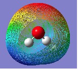
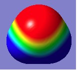
17. Click again on Surface Actions and then New Mapped Surface. The correct electrostatic potential surface should now be being visualised over your molecule. In the case of water, it appears as follows:


Manipulating the Surface
a) the charge range
1. At the top of the window visualising the electrostatic potential, there is a narrow bar showing colours ranging from red (negative) to blue (positive). At the ends of this bar are two numbers: in the case of the water molecule, these numbers are +/-5.493x10-2.
2. This bar is effectively the KEY to the electrostatic potential, indicating the charge that a certain colour on the electrostatic potential represents. The numbers, therefore, give the range of charge being displayed.
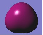
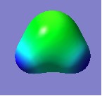
3. If, for example, you were to change this range to +/-5.493, you will find that the whole surface turns green (neutral):

4. This would be expected because the colours red and blue now represent charges of two orders of magnitude greater than actually present in a water molecule. Charges within a range of +/-5.493x10-2 would clearly fall into the green range shown on the colour bar.
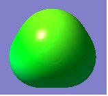
5. On the other hand, if the range is reduced to +/-2.493x10-2, the surface appears as follows:

6. Most of the water molecule holds charge greater than that given in this new range (more positive than +2.493x10⁻² or more negative than -2.493x10⁻²) and so the proportion of red or blue is much greater. Only a small curved band in the 'middle' of the molecule holds charge small enough to fall into the yellow/green/pale blue range on the colour bar.
b) the isovalue
1. The isovalue is effectively how 'far out' from the molecule you want to go to then visualise the electrostatic potential at the distance.
2. It can be changed by changing the value in the Density = box before visualising the potential energy surface (ie. before selecting New Mapped Surface from the Surface Actions drop-down menu). Remember to hide or remove any previous surfaces you have been looking at.
3. In the case of the water molecule, the default value is 0.000400. Increase this value to 0.05, and the electrostatic potential surface appears as follows:

4. The surface has clearly contracted considerably and you are now visualising the electrostatic potential much closer to the atoms' nuclei.
5. If the value is decreased to 9x10⁻⁶, the surface appears as follows:

6. The surface is now being visualised much further out. Indeed, it is so far out that in some areas, it is out of range of the data available and so 'holes' appear in the surface.
7. Changing the isovalue can be important for examining the interactions between two weakly coordinated molecules, for example.
c) the display format
1. As with visualising molecular orbitals, electrostatic potentials surfaces can also be visualized in mesh and transparent forms by right clicking on the molecule and selecting view, Display Format and then Surface.
2. You are also able to make holes in the surface to see the molecule inside. This is done by using the Z-clip found at the bottom of the window.
3. Click OK. An example is shown below: