When starting to model a system, some considerations about the particular calculations have to be made. A general approach to these will be given through the example of bulk Ag metals. General information on DFT can be found online and will not be discussed in this wiki. Some general information on Quantum Espresso and many resources can be found here. All the scripts and files described in this page can be found in the group's GitLab repository [1].

Parameter Optimisation

When studying a surface through modelling, the required accuracy of the calculation has to be determined. The accuracy is determined by the number of functions to expand the basis set into and number of K-points within the used grid. The number of expansion functions is determined by a maximum cut-off energy, which is set in the input file through the parameter ecutwfc and is given in Rydberg (Ry). To determine the necessary accuracy, calculations with different cut-off energies and K-points must be performed. The measure of accuracy can be chosen depending on the needs. In this case the total energy was used as the parameter to optimise the calculations for. A third parameter, the cut-off energy for the expansion of the electron density ecutrho, is set as to 10*ecutwfc as a good starting point. This parameter could also be optimised, but this was deemed unnecessary in this case. The three parameters are changed in the following sections of the input file found here:

&system
...
ecutwfc=28.0
ecutrho=280.0
...
K_POINTS { automatic }
8 8 8 1 1 1

In this example the calculation is performed with a wave function cut-off of 28.0 Ry and a k-point grid of size 8 in all dimensions. Running a calculation with this input gives an output file, from which total energy = -379.71040481 Ry can be extracted.

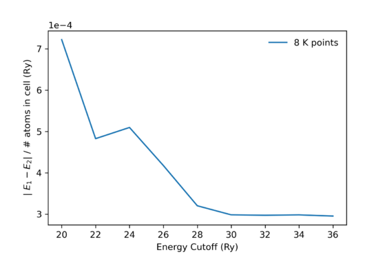
To optimise the calculation parameters the variation in total energy for different levels of calculation accuracy can be used. Increasing the calculations accuracy also results in a downwards trend of the total energy, that will show convergence above a threshold. To find this threshold the total energies are plotted against varied wave function cutoffs. One such plot is seen in Figure 1. The

This optimisation can also be performed for the amount of k-points used to sample the Brillouin zone (BZ). The input file contains the following section defining a grid of points where the BZ is sampled.

K_POINTS { automatic }
8 8 8 1 1 1

When using the 'automatic' option, the k-points will be automatically put in the form of a so called Monkhorst-Pack (MP) grid. This case specifies a 8x8x8 MP grid. The '1 1 1' is an option to choose the k-points with an offset from the center ( (0,0,0), also called Γ ) the BZ. The MP grid would be centered on Γ if not for the 1 1 1. The most simple grid would be only the Γ point specified with

K_POINTS { automatic }
1 1 1

When varying the density of the k-point grid, the following change in total energy can be observed:hen varying the