MRD:jt3818

This is an excellent report. The whole report is well-structured and makes efficient use of available formatting, making it easy and pleasant to read. Reasoning is supported with appropriate simulation results, which are presented in an easily reproducible way. Overall, it demonstrates a good understanding and engagement with the experiment. Well done! ⭐ Fdp18 (talk) 18:43, 24 May 2020 (BST)

Exercise 1

Transition State and the Potential Energy Surface

A transition state (TS) is a saddle point on the potential energy surface. The saddle point is a stationary point (zero gradient $\mathrm{\nabla }F=0$) which is is neither minimum nor maximum. The second partial derivative test can be used to identify a saddle point. For a two-variable functions, let $f(x,y)$ be a function of x and y, then $D=f_{xx}(x,y)f_{yy}(x,y)-f_{xy}^2(x,y)$:

1. If $D(a,b)>0$ and $f_{xx}(a,b)>0$, then a point (a,b) is a local minimum
2. If $D(a,b)>0$ and $f_{xx}(a,b)<0$, what about $f_{yy}(a,b)<0$? Fdp18 (talk) 18:14, 24 May 2020 (BST)

then a point (a,b) is a local maximum

1. If $D(a,b)<0$ then a point (a,b) is a saddle point
2. If $D(a,b)=0$, then the test is inconclusive.

Clean, understandable definitions with good use of formatting. Fdp18 (talk) 18:14, 24 May 2020 (BST)

For the multivariable functions, the test is defined in terms of the eigenvalues of the Hessian matrix.

1. If the Hessian is positive definite at a, then f has a local minimum at a.
2. If the Hessian is negative definite at a, then f has a local maximum at a.
3. If the Hessian has both positive and negative eigenvalues then a is a saddle point of f

Otherwise, the test is inconclusive.

Therefore, a local minimum can be distinguished from a saddle point using the second partial derivative test.

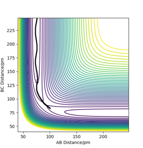
Figure 1a shows an example of the potential energy surface of the system of three hydrogen atoms in one line. The transition state is marked with a red cross in Figure 1b, where the two lines coming from the TS are eigenvectors of the Hessian matrix at the TS. The eigenvalues are −0.028 and 0.167 kJ·mol⁻¹·pm⁻², respectively. One eigenvalue is positive, one negative thus the considered point is really a saddle point. To be really picky here: You need to also show (or mention, at least) that this point is also a stationary point. Fdp18 (talk) 18:17, 24 May 2020 (BST)

• 
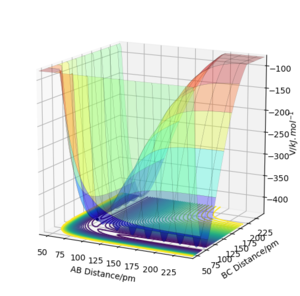  Figure 1 a) Surface plot of the PES for r_AB = r_BC =90.8 ppm
• 
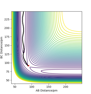
  b) Contour plot of the system from part a), the TS is marked with a red cross, the eigenvectors of the Hessian are the blue and red lines

Notation

The studied system consists of three hydrogen atoms labelled as A, B and C. Their relative internuclear disances are denoted as r_AB and r_BC, the angle between the lines connecting A—B and B—C was 180° for all simulations. The momenta of the couples AB and BC are denoted as p_AB and p_BC. Figure 2 illustrates the use of r_AB, r_BC.

OK, before I go on with commenting: I really like it that you properly define the complete geometry of your problem, including the nomenclature you use. And, although this might seem trivial, it is really good that you properly label your Figures and reference to them in your text. Fdp18 (talk) 18:20, 24 May 2020 (BST)

• 
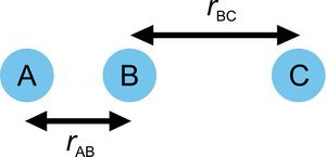  Figure 2 Notation of the coordinates

Trajectories from r_AB = r_BC to Locate the Transition State

To locate the TS, both internuclear distances were taken to be equal and the momenta were set to zero because the TS is expected to be centrosymmetrical and linear. Since the TS is a saddle point, there are no forces acting on the nuclei: $F=-\mathrm{\nabla }V=0$ where V is the potential energy. The nuclear separations were changed until the forces were close to zero. The separation in the TS was found to be r_AB = 90.8 ppm to 3 significant figures. The magnitude of the forces was 0.004 kJ·pm⁻¹·mol. Figure 1b which shows the countour plot with the TS designated with a cross (r_AB = r_BC =90.8 ppm, p_AB = p_BC = 0) and the variation of the internuclear distances AB, BC, CA is essentially constant (Figure 3).

The calculated bond length in TS is close to the literature value is 1.757 bohr (92.97 ppm), therefore the difference is only 3%.

Well done and well explained. I acknowledge that you even looked up a reference value for this TS, which is the first time I see someone doing that in a report for this experiment. Fdp18 (talk) 18:22, 24 May 2020 (BST)

• 
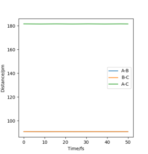  Figure 3 Distances vs Time plot for r_AB = r_BC =90.8 ppm

Calculating the reaction paths

The minimum energy path (MEP) connects the reactants and products via the path of minimum energy by resetting the velocities to zero at each step. MEP was generated starting from the point slightly displaced from the TS. It can be thought as a displacement from the unstable equilibtrium of the PES downhill in the direction of the steepest descent. The traced path is shown in Figure 4a, where the path is shown as a solid black line. It is evident also from the plot of the nuclei position against the time (Figure 4b), that there were no molecular vibrations and that atoms were smoothly changing their positions.

• 
  Figure 4 a) PES contour plot of the MEP calculation for r_AB = 91.8 ppm, r_BC =90.8 ppm, p_AB = p_BC = 0
• 
  b) Internuclear distances vs time for the system described in Figure 4a

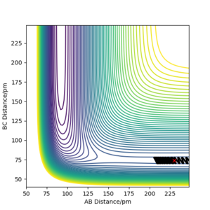
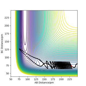
On the other hand, when the dynamics simulation was run, the formed H₂ molecule was vibrating thus the path depicting the nuclei motion in Figure 5a is more curvy due to the molecular vibrations. When the internuclear distances r_AB, r_BC were swapped, the particles were moving downhill in the direction to the second valley (Figure 5b, the trajectories are mirror images with respect to the diagonal of the plot). Then, the values of the positions and negative values of momenta from the last data points were run (obtained from the exported data) and the calculated trajectory (Figure 5c) is analogous to the one depicted by Figure 5b. Thus, the calculation is consistent as it gives a nearly the same trajectory for the reverse process.

• 
  Figure 5 a) PES contour plot for r_AB = 91.8 ppm, r_BC =90.8 ppm, p_AB = p_BC = 0
• 
  b) PES contour plot for r_AB = 90.8 ppm, r_BC =91.8 ppm, p_AB = p_BC = 0
• 
  c) PES contour plot for r_AB = 74 ppm, r_BC = 353 ppm, p_AB = 3.21 g·mol⁻¹·pm·fs⁻¹, p_AB = 5.10 g·mol⁻¹·pm·fs⁻¹

Reactive and Unreactive Trajectories

For a reaction to be successful, the reactants must have sufficient energy to go over over activation barrier (here the TS). The potential energy difference between the reactants (−434 kJ·mol⁻¹) and the transition state (−415 kJ·mol⁻¹) is 19 kJ·mol⁻¹ (literature value 23 kJ·mol⁻¹ ) equals the activation barrier if we consider the reaction classically (zero point energies ignored). Therefore, if the reactants have kinetic energy higher than 19 kJ·mol⁻¹, the reaction might proceed. Of course, the path does not need to go through the TS, it can go through any point on the critical dividing surface which is shown as a blue solid line in Figure 6.

In other words, the feasibility of the reaction H_AH_B + H_C → H_A + H_BH_C was analysed.

• 
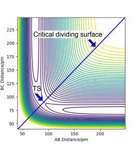  Figure 6 PES contour plot with highlighted crtical dividing surface

The table below shows the trajectories of 5 simulations with different intial momenta. Based on the values of the kinetic energies and shapes of the reaction paths, we can evalueate whether the trajectories are reactive or not.

p1/ g·mol−1·pm·fs−1	p2/ g·mol−1·pm·fs−1	Etot/kJ·mol−1	Reactive?	Description of the dynamics	Illustration of the trajectory
−2.56	−5.1	−414.3	Yes	The kinetic energy (19.5 kJ·mol-1) was sufficient for the reaction. The reactants passed the TS and the product was oscillating about the MEP.
−3.1	−4.1	−420.1	No	This system did not have enough kinetic energy (13.7 kJ·mol-1) thus the intially vibrating HAHB collided with approaching HC which was then reflected back.
−3.1	−5.1	−433.8	Yes	The system had enough kinetic energy to pass the activation barrier. Moreover, the HAHB was oscillating prior the collison and after passing TS, the formed molecule HBHC was oscillating with larger amplitudes. Thus, it can be expected that the product was in an excited vibrational level.
−5.1	−10.1	−357.3	No	Although the molecule had sufficient kinetic energy, it passed through the dividing surface twice and the reactants were regenerated. It should be noted that the HAHB molecule was not vibrating before the collision, then the temporary molecule HBHC was vibrating with large amplitudes until it reformed the vibrationally excited molecule HAHB and atom HC
−5.1	−10.6	−349.5	Yes	Similar to the previsous case but the kinetic energy was even higher. The trajectory pierced the critical dividing surface three time and the vibrationally excited molecule HBHC was formed.

Well done so far, nothing to complain about. Fdp18 (talk) 18:27, 24 May 2020 (BST)

Transition State Theory

Transition state theory (TST), also known as activated-complex theory, was devolped in 1930s by Pelzer, Wigner, Polanyi and Eyring. TST allows the computation of the reaction rates by considering the regions of reactants and the region of TS on the PES without having to calculate the reaction trajectories. It is based on several assumptions:

1. All the supermolecules ('combined reactants') that cross the critical dividing surface become products.
2. During the reaction, the Boltzmann distribution of energy of the reactants is maintaned.
3. The supermolecules crossing the critical surface from the reactant side have a Boltzmann distribution of energy corresponding to the temperature of the reacting system.
4. The transition state is in the quasiequilibrium with the reactants.
5. Born-Oppenheimer approximation is valid — vibrational, rotataional, translational and electronic transitions/levels can be considered independently. The "Born-Oppenheimer" approximation encompasses only the separation of nuclear and electronic motions. i.e. the (much) lighter particles are thought to adjust/relax immediately. Fdp18 (talk) 18:30, 24 May 2020 (BST)

When comparing these assumptions with the results of reactive and unreactive trajectories, it is evident, that the system can pass through the diving surface but the reaction is unsuccessful - this decreases the calculated rate. Also, this theory ignores the quantum mechanical tunneling through the barrier which is not negligible for light particles such as proton and electron, thus this also underestimates the rate. Despite these limitations, the TST predicts the rate constants within the same order of magnitude.

Exercise 2

Locating the Transition State

The reaction F + H₂ → HF + H is highly exothermic. Using the Hammonds postulate, we can expect that the reaction would have an early transition state, i.e. the structure will resemble the reactants. The reaction coordinate is illustrated in Figure 7a with the highligted activation barriers for the forward and reverse reactions. Thus, it can be expected that the H⏤H distance will be similar to H₂ molecule (74.1 ppm ) and that the approaching F atom would be relatively far from the H⏤F distance as in HF molecule (91.7 ppm ). The different internuclear distances were tested until the the forces along AB and BC (with respect to labelling of the atoms as in the previous exercise) were close to zero (0.000 and −0.003 kJ·mol⁻¹·pm⁻¹). The eigenvalues of the Hessian matrix were −0.002 and 0.332 kJ·pm⁻²·mol⁻¹, therefore, the considered point is a saddle point. The found internuclear distances were r_AB =180.9 ppm, r_BC =74.5 ppm where A=fluorine, B=C=hydrogen. The controur plot with the highlighted TS and the surface plot of the PES are shown in Figure 7b, 7c.

The calculated structure of the TS is similar to the literature values r_AB =167.7 ppm, r_BC =75.2 ppm.

• 
  Figure 7 a) The illustration of the reaction coordinate with the approximate structure of the TS and highlighted activation energies E_a,1, E_a,-1
• 
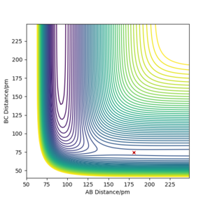  b) PES contour plot for r_AB =180.9 ppm, r_BC =74.5 ppm, p_AB = p_BC = 0. The TS is highlighted with a red cross.
• 
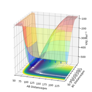  c) PES surface plot, parameters same as in Figure 7b.

Your schemes are really nice, and the explanation is clear, concise, complete and easy to follow. Well done. Fdp18 (talk) 18:34, 24 May 2020 (BST)

Activation Energies

To estimate the classical reaction barriers (e.g. by ignoring the zero point energies), the structure of TS was perturbed by 1 ppm in either direction so the reaction went downhill back to the reactants or to the products. This was carried out by performing the MEP calculation with 5000 steps. The contour plots of the PES and the potential energy vs time plots are in Figure 8a-d. The stepsize for the forward reaction was increased to 0.5 from 0.1 fs so that the potential energy in Figure 8b could reach plateaou faster. The activation energies were 1.1 and 126 kJ·mol⁻¹, respectively. Experimental values for the activation barriers are 6–10 and 135 kJ·mol⁻¹.

• 
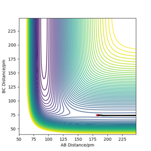  Figure 8 a) Forward reaction: MEP for r_AB =181.9 ppm, r_BC =74.5 ppm, p_AB = p_BC = 0
• 
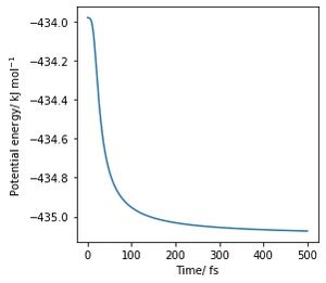  b) Potential energy agains time for the forward reaction, activation barrier: 1.1 kJ·mol⁻¹
• 
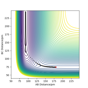  c) Backward reaction: MEP for r_AB =179.9 ppm, r_BC =74.5 ppm, p_AB = p_BC = 0
• 
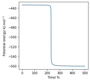  d) Potential energy agains time for the backward reaction, activation barrier: 126 kJ·mol⁻¹

No issues here. Fdp18 (talk) 18:35, 24 May 2020 (BST)

Reaction Dynamics

An example of the reaction trajectory is shown in Figure 10. The reaction is highly exothermic which means that some energy has to be released by converting either to translational, vibrational or rotational. The reactant H₂ is initially in a low vibrational level (most probably the ground state) and the produced HF is evidently in an excited level due to the high amplitudes of the vibrations. Most likely, the light in the infrared region would be then emitted stemming from the transition between the first excited and the ground vibrational state. To which vibrational level was HF excited can be studied, for example, using infrared chemiluminescence spectroscopy.

F + H₂

As can be seen in Figure 9a-f, when the intial momentum of HF was kept constant (p_AB = −1 g·mol⁻¹·pm·fs⁻¹) and the initial momentum of HH varied between −6.1 and 6.1 g·mol⁻¹·pm·fs⁻¹, most of the trajectories were unreactive. Although each system had enough kinetic energy to pass the activation barrier, only one of the six shown actually did. These systems have in common that they have the kinetic energy mostly stored in the vibrational motion.

• 
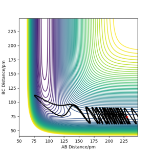  Figure 9 a) Contour plot of PES for r_AB = 230 ppm, r_BC =74 ppm, p_AB = −1 g·mol⁻¹·pm·fs⁻¹, p_BC = −6.1 g·mol⁻¹·pm·fs⁻¹
• 
  b)r_AB = 230 ppm, r_BC =74 ppm, p_AB = −1 g·mol⁻¹·pm·fs⁻¹, p_BC = −4 g·mol⁻¹·pm·fs⁻¹
• 
  c) r_AB = 230 ppm, r_BC =74 ppm, p_AB = −1 g·mol⁻¹·pm·fs⁻¹, p_BC = −1 g·mol⁻¹·pm·fs⁻¹
• 
  d) r_AB = 230 ppm, r_BC =74 ppm, p_AB = −1 g·mol⁻¹·pm·fs⁻¹, p_BC = 1 g·mol⁻¹·pm·fs⁻¹
• 
  e) r_AB = 230 ppm, r_BC =74 ppm, p_AB = −1 g·mol⁻¹.pm·fs⁻¹, p_BC = 4 g·mol⁻¹·pm·fs⁻¹
• 
  f) r_AB = 230 ppm, r_BC =74 ppm, p_AB = −1 g·mol⁻¹·pm·fs⁻¹, p_BC = 6.1 g·mol⁻¹·pm·fs⁻¹

On the other hand, when the initial momenta were changed to p_AB = −1.6 g·mol⁻¹·pm·fs⁻¹ and p_BC = 0.2 g·mol⁻¹·pm·fs⁻¹, less kinetic energy was stored as vibrations and more as translational. Figure 10 shows the trajectory for this system which was successful.

• 
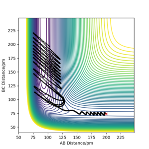  Figure 10 Contour plot of PES for r_AB = 200 ppm, r_BC =74 ppm, p_AB = −1.6 g·mol⁻¹·pm·fs⁻¹, p_BC = 0.2 g·mol⁻¹·pm·fs⁻¹

H + HF

For the reverse reaction, which is endothermic, it was more difficult to find initial conditions that would lead to reactive trajectories. Figure 11a, b show two successful trajectories — the first one depicts the H—H couple which had high value of the momentum corresponding to high translational energy, while in the second one, HF was in an excited vibrational state.

• 
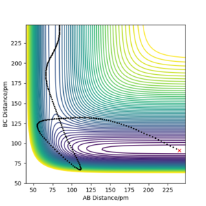  Figure 11a) Contour plot of PES for r_AB = 240 ppm, r_BC = 91 ppm, p_AB = −20 g·mol^-1·pm·fs^-1, p_BC = 0.02 g·mol^-1·pm·fs^-1
• 
  b) Contour plot of PES for r_AB = 240 ppm, r_BC = 91 ppm, p_AB = −1 g·mol^-1·pm·fs^-1, p_BC = −23 g·mol^-1·pm·fs^-1

Good use of figures and examples to support your reasoning, even with the starting conditions given. Fdp18 (talk) 18:38, 24 May 2020 (BST)

Polanyi's rules

The relative efficiencies of promoting the reactions in terms of translational and vibrational modes were described by M. Polanyi:

1. For an early TS (reactant-like TS), translational activation is more effective for overcoming the activation barrier.
2. For a late TS (product-like TS), vibrational excitation is more efficient.

Thus, the plots in the previous sections agree with the Polanyi‘s empiral rules. The reaction of F and H₂ is highly exothermic and thus has a reactant-like TS. Indeed, the reactants in Figure 10a-f were vibrationally activated and most trajectories were unreactive while when the reactants had enough translational energy (Figure 11), the reaction proceeded to form a vibrationally excited HF and H. On the other hand, H + HF reaction is endothermic and has a product-like TS. Therefore, as it can be seen in Figure 12a,b, both activation were feasible, but it was easier to find the reactive trajectories with vibrationally activated HF (not all the trajectories are shown here).

We can think about this problem classically by treating the reaction as a frictionless movement of the mass traced by the trajectory on the PES. PES energy surface of one successful trajectory is shown in Figure 12a,b rotated from two sides. One side showns the endothermic reaction (H + HF) while the other the exothermic (F + H₂). From Figure 12a it seems natural that when the reactants vibrate strongly, it might be efficient way to surmount the barrier. Conversely, in the exothermic direction, only sufficient amount of translational energy is needed so that from as the activated complex is formed, the trajectory that drops downhill. Thus, the trajectory has to be in the correct uphill direction so that the mass would not bounce back. We may view it as an example of the principle of microscopic reversibility.

Excellent reasoning, this paragraph shows very well that you understood the underlying material. Fdp18 (talk) 18:40, 24 May 2020 (BST)

• 
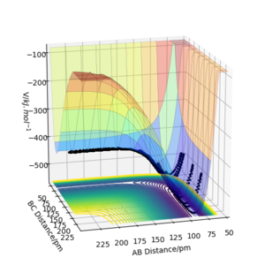  Figure 12a) Surfaceplot of PES for r_AB = 230 ppm, r_BC = 74 ppm, p_AB = −1.6 g·mol^-1·pm·fs^-1, p_BC = 0.2
• 
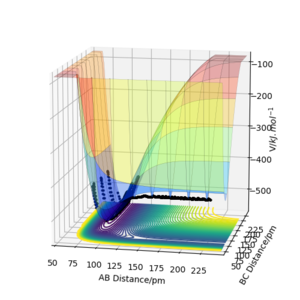  b) Same parameters as in a), but from a different point of view.

References

- ↑ Mielke, S. L.; Schwenke, D. W.; Peterson, K. A. Benchmark Calculations of the Complete Configuration-Interaction Limit of Born–Oppenheimer Diagonal Corrections to the Saddle Points of Isotopomers of the H+H2 Reaction. The Journal of Chemical Physics 2005, 122 (22), 224313. doi.org/10.1063/1.1917838
- ↑ 2.0 2.1 2.2 2.3 Levine, Ira N. Physical Chemistry. 6th ed., McGraw-Hill, 2009, pp. 880-902
- ↑ 3.0 3.1 3.2 3.3 3.4 Moss, S. J.; Coady, C. J. Potential-Energy Surfaces and Transition-State Theory. Journal of Chemical Education 1983, 60 (6), 455. doi.org/10.1021/ed060p455
- ↑ 4.0 4.1 Cccbdb.nist.gov. 2020. Computational Chemistry Comparison And Benchmark Database. [online] Available at: https://cccbdb.nist.gov/introx.asp [Accessed 22 May 2020].
- ↑ Polanyi, J. C. Concepts in Reaction Dynamics. Accounts of Chemical Research 1972, 5 (5), 161–168. . doi.org/10.1021/ar50053a001