MRD:ZZY15

Overall: A bit rushed and in terms of the science, needs a little work with heat capacity. Have a think about your report style before your start your MSci/BSc project. Reading papers helps! Also your grammar needs a lot of work - the centre for Academic English is an excellent facility. Be careful about units!! Mark:50/100

Molecular dynamics simulations of simple liquids

Abstract

This abstract is pretty poor... The purpose of an abstract is to summarise the purpose of your work, the data you obtained during your work and the conclusions you've taken home from it. You haven't really done any of that here and there are a number of grammar errors. Too rushed!

This wiki report investigate gram the structural and thermodynamic properties of physical systems using computer simulations.this sentence is really vague... The generation of computer simulation is shown.what does this even mean? The variance of properties gram such as heat capacity and diffusion coefficient in different phases was studied.

Introduction

This introduction is really quite weak. The introduction should provide concrete research to support either a broad reaching or specific interest to your work i.e show your niche. This is a really nice paper with relevance to this work https://doi.org/10.4271/932811 - in this lab we concentrate on commenting on the diffusion and dynamic properties of phase. This paper they talk about this and how it varies with temperature/pressure. Your style needs some work before your MSci/BSc project and I would advise you visit the Centre for Academic English because your English needs some work.

Liquid plays gram a vital role in all living organisms, it is where life is evolved from. life is evolved from living organisms? What are you trying to say? The behavior of liquid gram such as its thermodynamic, structure and motion has always been fascinating to the scientific world. avoid sweeping statements like this... they serve literally no purpose. The study of liquid gram has a long history, from observation of Brownian motion to neutron scattering experiments. this sentence also serves no purpose... Beside gram all the work done to experimentally understand the structure and dynamics of liquid, scientists would you not class yourself in this category? have worked hard to construct models for simple liquid gram to investigate its behavior. Earlier works use physical model gram to approach this. what sort of physical model? This is too vague. Further improvement is gram to use a mathematics model instead and do analysis using computer. improvement to what? Computer simulation gram of molecular dynamics is an effective way to monitor thermodynamic properties of liquid. In this experiment, we use computer simulations to solve the equation gram of motion for a set of Lennard-Jones particles. More complex simulations can be preformed gram by change variables and settings to investigate details of molecular motion and structure in reactions that are hard to probe experimentally, such as enzyme action, heterogeneous catalysis etc.uncited and again serving no purpose...

Aims and Objectives

In this experiment, we perform molecular dynamic simulations on the computer would be impressed if you did it with pen and paper. in order to calculate both structural and dynamic properties of a simple liquid. We use the computer simulation to provide results for problems in statistical mechanics what problems in statistical mechanics? which are then compared with experimental results or theoretical predictions. First we want to investigate how far the system is able to fluctuate from its average equilibrium state are we doing this here?, in order to do that, the heat capacity of the system in different density-temperature phases was calculated. Second we want to reproduce the structural features of different phases, the radial distribution function was calculated to have an insight gram. Lastly, we want to know how much the atoms in our simulation move around too colloquial, the diffusion coefficient of different phases which calculated gram from MSD and VACF was used to characterize it.

Methods

In this experiment, all the molecular dynamic simulations were ran gram by the high performance computing system of college. The model used for simulation is the Lennard-Jones potential with timestep = 0.0025 for how long were we simulating the system?. The Verlet Algorithm No, the velocity-Verlet algorithm was used... hence our step didn't rely on the previous was used to approximate numerical solutions for each timestep, such as position, velocity, energy etc. For the results to be more manageable, all quantities obtained were in reduced unit.

The input file for simulation firstly build gram a box containing several hundreds of lattice unit cells how many?. Atoms within that box were used for simulation I would never have guessed!. The input file also specifies the use of Lennard-Jones potential, its cutoff(equals to 3.00 2 what? 3 sigma!) and its parameters (both equal to 1) which parameters? Specify them! Sigma and epsilon.. Also, conditions such as temperature, pressure, density etc. never use etc in a report of the simulation box can be varied in the input file to obtain desired quantities under different conditions. The HPC gave output file as log file and trajectory file gram. The log file contains all the numerical solutions, the trajectory file can be viewed in a programme called VMD, which displays the simulation box.

The phase diagram for the Lennard-Jones system was used to obtain the density and temperature parameters for different phases to calculate the radial distribution function, mean squared displacement and the velocity autocorrelation function of different phases. citation? In addition, the lattice type for solid is face-centered cubic instead of simple cubic for liquid and gas.

Table 1. Parameters used in reduced unit for different phases.

	Gas	Liquid	Solid
Temperature	1.2	1.2	1.2
Density	0.05	0.8	1.3

Results and Discussion

The idea was that you write a coherent report (without tasks!)

Theory

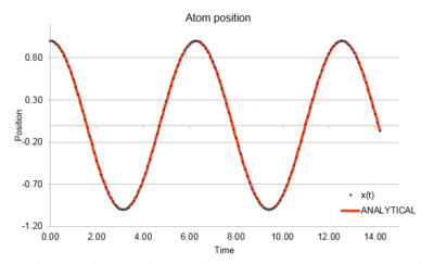
Task 1 Open the file HO.xls. In it, the velocity-Verlet algorithm is used to model the behaviour of a classical harmonic oscillator. Complete the three columns "ANALYTICAL", "ERROR", and "ENERGY": "ANALYTICAL" should contain the value of the classical solution for the position at time $t$, "ERROR" should contain the absolute difference between "ANALYTICAL" and the velocity-Verlet solution (i.e. ERROR should always be positive -- make sure you leave the half step rows blank!), and "ENERGY" should contain the total energy of the oscillator for the velocity-Verlet solution. Remember that the position of a classical harmonic oscillator is given by $x\left(t\right)=A\cos (\omega t+\varphi )$ ($A$ = 1.00, $\omega$ = 1.00, and $\varphi$ = 0.00).

Figure 1:Atom Position versus Time.

Figure 2:Energy versus Time at time-step 0.1.

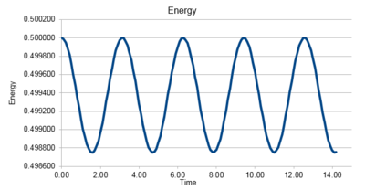The velocity-Verlet solution is very close to the classical solution, showing that the velocity-Verlet algorithm is a good method for integrating Newton's motion.

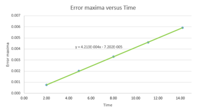
Task 2 For the default timestep value, 0.1, estimate the positions of the maxima in the ERROR column as a function of time. Make a plot showing these values as a function of time, and fit an appropriate function to the data.

Figure 3:Max error versus Time.

would be nice to plot this on the same graph as your error

The error increases linearly with time, indicating the difference between analytical data and velocity-Verlet solution increases over time. This is because the velocity-Verlet algorithm use value from last timestep to estimate new value, the error builds up.

Task 3 Experiment with different values of the timestep. What sort of a timestep do you need to use to ensure that the total energy does not change by more than 1% over the course of your "simulation"? Why do you think it is important to monitor the total energy of a physical system when modelling its behaviour numerically?

Figure 4:Energy versus Time at time-step 0.15.

Figure 5:Energy versus Time at time-step 0.2.

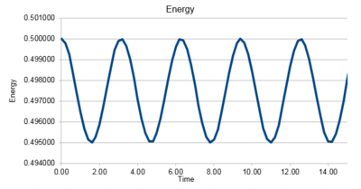0.2 is the largest timestep that can be used, the total energy change close to 1%. Monitoring energy of the system gives an idea of whether the data obtained is accurate throughout the simulation and it also shows the change of system throughout the simulation. tick

Task 4 For a single Lennard-Jones interaction, $\varphi \left(r\right)=4ϵ(\frac{{\sigma }^{12}}{r^{12}}-\frac{{\sigma }^6}{r^6})$, find the separation, $r_0$, at which the potential energy is zero. What is the force at this separation? Find the equilibrium separation, $r_{eq}$, and work out the well depth ($\varphi \left(r_{eq}\right)$). Evaluate the integrals $\underset{2\sigma }{\overset{\mathrm{\infty }}{\int }}\varphi \left(r\right)\mathrm{d}r$, $\underset{2.5\sigma }{\overset{\mathrm{\infty }}{\int }}\varphi \left(r\right)\mathrm{d}r$, and $\underset{3\sigma }{\overset{\mathrm{\infty }}{\int }}\varphi \left(r\right)\mathrm{d}r$ when $\sigma =ϵ=1.0$.

$\varphi \left(r_0\right)$ = 0 $4ϵ(\frac{{\sigma }^{12}}{r_0^{12}}-\frac{{\sigma }^6}{r_0^6})$ = 0

$\frac{{\sigma }^{12}}{r_0^{12}}=\frac{{\sigma }^6}{r_0^6}$

$r_0=\sigma$

$\frac{\mathrm{d}\varphi \left(r\right)}{\mathrm{d}r}=4ϵ(-12\frac{{\sigma }^{12}}{r^{13}}+6\frac{{\sigma }^6}{r^7})$

When $\frac{\mathrm{d}\varphi \left(r\right)}{\mathrm{d}r}$ = 0

$(-12\frac{{\sigma }^{12}}{r^{13}}+6\frac{{\sigma }^6}{r^7})$ = 0

$12\frac{{\sigma }^{12}}{r^{13}}=6\frac{{\sigma }^6}{r^7}$

$r_{eq}=\sqrt[6]{2}\sigma$

$\varphi \left(r_{eq}\right)=4ϵ(\frac{{\sigma }^{12}}{(\sqrt[6]{2}\sigma {)}^{12}}-\frac{{\sigma }^6}{(\sqrt[6]{2}\sigma {)}^6})$

$\varphi \left(r_{eq}\right)=-ϵ$tick

When $\sigma =ϵ=1.0$

$\int \varphi \left(r\right)\mathrm{d}r=\int 4(\frac{1}{r^{12}}-\frac{1}{r^6})\mathrm{d}r=-\frac{4}{11r^{11}}+\frac{4}{5r^5}$

$\underset{2\sigma }{\overset{\mathrm{\infty }}{\int }}\varphi \left(r\right)\mathrm{d}r=-0.02482$tick

$\underset{2.5\sigma }{\overset{\mathrm{\infty }}{\int }}\varphi \left(r\right)\mathrm{d}r=-0.00818$tick

$\underset{3\sigma }{\overset{\mathrm{\infty }}{\int }}\varphi \left(r\right)\mathrm{d}r=-0.00329$tick

Task 5 Estimate the number of water molecules in 1ml of water under standard conditions. Estimate the volume of 10000 water molecules under standard conditions.

Number of water molecules in 1mL of water = $3.342\times 10^{22}$tick

Volume of 10000 water molecules = $2.989\times 10^{-19}\mathrm{m}\mathrm{L}$tick

Task 6 Consider an atom at position (0.5, 0.5, 0.5) in a cubic simulation box which runs from (0, 0, 0) to (1, 1, 1). In a single timestep, it moves along the vector (0.7, 0.6, 0.2). At what point does it end up, after the periodic boundary conditions have been applied?

Atom at position (0.5, 0.5, 0.5) moves along the vector (0.7, 0.6, 0.2) ends at position (1.2, 1.1, 0.7). After the periodic boundary conditions have been applied, the position of the atom is (0.2, 0.1, 0.7).

Task 7 The Lennard-Jones parameters for argon are $$\begin{gathered} \sigma =0.34\mathrm{n}\mathrm{m},ϵ \\ / \\ {k}_B=120\mathrm{K} \end{gathered}$$. If the LJ cutoff is $r^{*}=3.2$, what is it in real units? What is the well depth in $$\begin{gathered} {\mathrm{k}\mathrm{J} \\ \mathrm{m}\mathrm{o}\mathrm{l}}^{-1} \end{gathered}$$? What is the reduced temperature $T^{*}=1.5$ in real units?

$r=\sigma \times r^{*}=0.34\times 3.2=1.088\mathrm{n}\mathrm{m}$

$T=\frac{T^{*}ϵ}{k_B}=1.5\times 120=180\mathrm{K}$

$$\begin{gathered} \varphi \left(r_{eq}\right)=-ϵ=-0.9977{\mathrm{k}\mathrm{J} \\ \mathrm{m}\mathrm{o}\mathrm{l}}^{-1} \end{gathered}$$tick

Equilibration

Task 1 Why do you think giving atoms random starting coordinates causes problems in simulations? Hint: what happens if two atoms happen to be generated close together?

If two atoms are placed close together, they may repel each other with a large force and hence, generating a large temperature spike.

Task 2 Satisfy yourself that this lattice spacing corresponds to a number density of lattice points of 0.8. Consider instead a face-centred cubic lattice with a lattice point number density of 1.2. What is the side length of the cubic unit cell?

Each simple cubic lattice has one lattice point.

Number density of lattice points $=\frac{1}{1.07722^3}=0.8$tick

Each face-centred cubic lattice has four lattice points.

Number density of lattice points $=\frac{4}{x^3}=1.2$tick

$x^3=\frac{4}{1.2}$

Side length of the cubic unit cell $x=1.4938$tick

Task 3 Consider again the face-centred cubic lattice from the previous task. How many atoms would be created by the create_atoms command if you had defined that lattice instead?

4000 atoms would be created.

Task 4 Using the LAMMPS manual, find the purpose of the following commands in the input script:

mass 1 1.0
pair_style lj/cut 3.0
pair_coeff * * 1.0 1.0

The mass of type 1 atom is 1.0. The potential function used is Lennard-Jones potential with cutoff distance = 3.0, $\sigma$ = 1.0, $ϵ$ = 1.0.

Task 5 Given that we are specifying ${\mathbf{x}}_i\left(0\right)$ and ${\mathbf{v}}_i\left(0\right)$, which integration algorithm are we going to use?

The velocity verlet algorithm is used.

Task 6 Look at the lines below.

### SPECIFY TIMESTEP ###
variable timestep equal 0.001
variable n_steps equal floor(100/${timestep})
timestep ${timestep}

### RUN SIMULATION ###
run ${n_steps}
run 100000

The second line (starting "variable timestep...") tells LAMMPS that if it encounters the text ${timestep} on a subsequent line, it should replace it by the value given. In this case, the value ${timestep} is always replaced by 0.001. In light of this, what do you think the purpose of these lines is? Why not just write:

timestep 0.001
run 100000

These lines defined two variables: timestep and n_steps, which can be called later. Defining variables makes changing settings easier. Because only the define variables lines needs change instead of changing all the value in the input file.

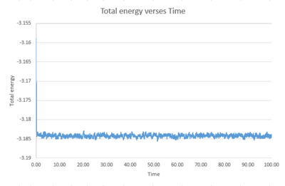
Task 7 Make plots of the energy, temperature, and pressure, against time for the 0.001 timestep experiment (attach a picture to your report). Does the simulation reach equilibrium? How long does this take? When you have done this, make a single plot which shows the energy versus time for all of the timesteps (again, attach a picture to your report). Choosing a timestep is a balancing act: the shorter the timestep, the more accurately the results of your simulation will reflect the physical reality; short timesteps, however, mean that the same number of simulation steps cover a shorter amount of actual time, and this is very unhelpful if the process you want to study requires observation over a long time. Of the five timesteps that you used, which is the largest to give acceptable results? Which one of the five is a particularly bad choice? Why?

Figure 6:Energy versus time for 0.001 timestep.

Figure 7:Temperature versus time for 0.001 timestep.

Figure 8:Pressure versus time for 0.001 timestep.

The simulation for the 0.001 timestep reaches equilibrium at around 0.45.

Figure 9:Energy versus time.

All timesteps other than 0.015 reach equilibrium. 0.015 is a bad choice as the energy, instead of reaching equilibrium, increases over time. The largest timestep to give acceptable results is 0.0025 as it has similar energy trend to the 0.001 timestep.

Running simulations under specific conditions

Task 1 We need to choose $\gamma$ so that the temperature is correct $T=\mathfrak{𝔗}$ if we multiply every velocity $\gamma$. We can write two equations:

$\frac{1}{2}\sum _i{m}_i{v}_i^2=\frac{3}{2}N{k}_{B}T$

$\frac{1}{2}\sum _i{m}_i{\left(\gamma v_i\right)}^2=\frac{3}{2}N{k}_B\mathfrak{𝔗}$

Solve these to determine $\gamma$.

$\frac{1}{2}\sum _i{m}_i{\left(\gamma v_i\right)}^2={\gamma }^2\frac{1}{2}\sum _i{m}_i{v}_i^2={\gamma }^2\frac{3}{2}N{k}_{B}T$

$\gamma =\sqrt{\frac{\mathfrak{𝔗}}{T}}$ tick

Task 2 Use the manual page to find out the importance of the three numbers 100 1000 100000. How often will values of the temperature, etc., be sampled for the average? How many measurements contribute to the average? Looking to the following line, how much time will you simulate?

100, 1000 and 100000 are N_every, N_repeat and N_freq respectively. The data will be sampled for average every 10000 timesteps. 100 measurements contribute to the average. 1000 averages will be taken to calculate the total average of the data.

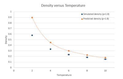
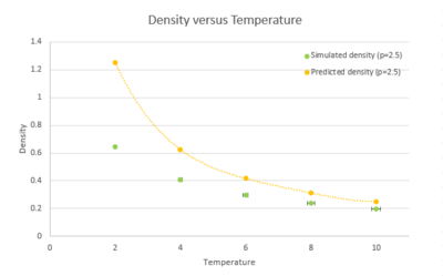
Task 3 When your simulations have finished, download the log files as before. At the end of the log file, LAMMPS will output the values and errors for the pressure, temperature, and density $\left(\frac{N}{V}\right)$. Use software of your choice to plot the density as a function of temperature for both of the pressures that you simulated. Your graph(s) should include error bars in both the x and y directions. You should also include a line corresponding to the density predicted by the ideal gas law at that pressure. Is your simulated density lower or higher? Justify this. Does the discrepancy increase or decrease with pressure?

Figure 10:Density versus temperature (P=1.8).

Figure 11:Density versus temperature (P=2.5).

At different The density decreases with temperature for both pressures. The predicted density ideal gas is always higher than density from simulation and the discrepancy between them decreases with temperature. tick This is because the ideal gas law ignore the neglects gram both molecular size and intermolecular attractions, leading to higher density than real gas system as molecules can be very close to each other. tick While as the Lenard-Jones gram system takes into account the repulsion between molecules. The increase in temperature results in greater velocity of molecules, therefore less molecules needed to maintain the same pressure per unit volume, the density decreases. At high temperature and low pressure, molecules are more diffuse and the interaction between them becomes less pronounced, they behave more like ideal gas. This explains the decrease of discrepancy with temperature, also the smaller discrepancy with lower pressure.tick, this is concise - not a bad explanation!

Calculating heat capacities using statistical physics

Task 1 As in the last section, you need to run simulations at ten phase points. In this section, we will be in density-temperature $({\rho }^{*},T^{*})$ phase space, rather than pressure-temperature phase space. The two densities required at $0.2$ and $0.8$, and the temperature range is $2.0,2.2,2.4,2.6,2.8$. Plot $C_V/V$ as a function of temperature, where $V$ is the volume of the simulation cell, for both of your densities (on the same graph). Is the trend the one you would expect? Attach an example of one of your input scripts to your report.

$C_V=\frac{\partial E}{\partial T}=\frac{\mathrm{V}\mathrm{a}\mathrm{r}\left[E\right]}{k_B{T}^2}=N^2\frac{⟨E^2⟩-{⟨E⟩}^2}{k_B{T}^2}$

Figure 12:Heat capacity/volume versus temperature.

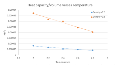
The heat capacity per unit volume is higher for higher density. Higher density means there are more molecules per unit volume, leading to higher density of states and more degree of freedom. According to the equipartition theorem, more energy needed for the same temperature raise, in other words, the heat capacity is larger. For both densities, the heat capacity per unit volume decreases with temperature. This is because for the same density of states, at higher temperature, populating of higher energy states becomes easier. Therefore the heat capacity decreases. This inverse relationship is more pronounced for higher density, as higher density of states.

Example of input script:

### DEFINE SIMULATION BOX GEOMETRY ###
variable dens equal 0.2
lattice sc ${dens}
region box block 0 15 0 15 0 15
create_box 1 box
create_atoms 1 box

### DEFINE PHYSICAL PROPERTIES OF ATOMS ###
mass 1 1.0
pair_style lj/cut/opt 3.0
pair_coeff 1 1 1.0 1.0
neighbor 2.0 bin

### SPECIFY THE REQUIRED THERMODYNAMIC STATE ###
variable T equal 2.0
variable timestep equal 0.0025

### ASSIGN ATOMIC VELOCITIES ###
velocity all create ${T} 12345 dist gaussian rot yes mom yes

### SPECIFY ENSEMBLE ###
timestep ${timestep}
fix nve all nve

### THERMODYNAMIC OUTPUT CONTROL ###
thermo_style custom time etotal temp press
thermo 10

### RECORD TRAJECTORY ###
dump traj all custom 1000 output-1 id x y z

### SPECIFY TIMESTEP ###

### RUN SIMULATION TO MELT CRYSTAL ###
run 10000
unfix nve
reset_timestep 0

### BRING SYSTEM TO REQUIRED STATE ###
variable tdamp equal ${timestep}*100
fix nve all nve temp ${T} ${T} ${tdamp} 
run 10000
reset_timestep 0

### MEASURE SYSTEM STATE ###
thermo_style custom atoms etotal temp vol
variable etotal equal etotal
variable etotal2 equal etotal*etotal
variable temp equal temp
variable temp2 equal temp*temp
variable atoms equal atoms
variable atoms2 equal atoms*atoms
variable volume equal vol
fix aves all ave/time 100 1000 100000 v_temp v_temp2 v_etotal v_etotal2
run 100000

variable avetemp equal f_aves[1]
variable avetemp2 equal f_aves[2]
variable aveetotal equal f_aves[3]
variable aveetotal2 equal f_aves[4]
variable heatcapacity equal ${atoms2}*(${aveetotal2}-${aveetotal}*${aveetotal})/${avetemp2}

print "Averages"
print "--------"
print "Temperature: ${avetemp}"
print "Temperature2: ${avetemp2}"
print "aveetotal: ${aveetotal}"
print "aveetotal2: ${aveetotal2}"
print "volume: ${volume}"
print "heatcapacity: ${heatcapacity}"

Structural properties and the radial distribution function

Task 1 Perform simulations of the Lennard-Jones system in the three phases. When each is complete, download the trajectory and calculate $g(r)$ and $\int g(r)\mathrm{d}r$. Plot the RDFs for the three systems on the same axes, and attach a copy to your report. Discuss qualitatively the differences between the three RDFs, and what this tells you about the structure of the system in each phase. In the solid case, illustrate which lattice sites the first three peaks correspond to. What is the lattice spacing? What is the coordination number for each of the first three peaks?

Figure 13:g(r) versus r.

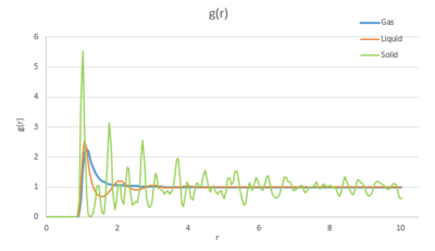
At first, the RDF is zero for a small range of R. This corresponds to the effective width of the atom. This is the centre-centre distance The three RDF graphs all have a sharp peak after the zero region then decay to 1 with oscillations. However, the intensities of peaks decrease from solid to gas, so does the interval between subsequent peaks. For solid, which has higher density, atoms are more closely packed and have a long-term ordering pattern, therefore there are subsequent peaks occurring in roughly the same interval. However, the subsequent peaks are much smaller due to repulsion from the first sphere.not quite... reduction in the peak height is a manifestation of less order at greater radial distances As for liquid, the atoms are more diffuse and need to go further to encounter another atom, there are no exact interval between peaks. what about the small, smooth peaks? Why are they smooth? The RDF for gas only has one peak, showing a single coordination sphere as gas atoms are the most diffuse, there are no clear subsequent coordination spheres.tick In addition, the peaks for solid are more sharp compare to liquid and gas, this indicates the thermal motion of atoms vibration around their lattice site is smaller for solid. The broadened peaks for liquid and gas correspond to larger vibrations. The RDFs eventually go to 1 for liquid and gas systems, which means the local density would be equal to the mean density $\rho$ at large value of r for diffuse systems.

$\rho (r)={\rho }^{bulk}g(r)$

The reason for this is that the atoms become independent at large distance, the interactions between them, which affect g(r), become zero. The systems turn into ideal. ? this doesn't make sense The gas system reach ideality fastest as it's the most diffuse system and the intermolecular interaction is negligible beyond the first coordination shell.

$g(r)=\exp [-\frac{u(r)}{kT}]$

Figure 14:int(g(r)) versus r for solid.

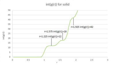
The first three peaks in the solid graph correspond to the first three coordination shells (or solvation shells) the reference particle encounters. The coordination number for each peak is 12, 6, 24 respectively, which is consistent to the fcc lattice predication. Lattice spacing is around 0.35(0.119 nm).tick

Dynamical properties and the diffusion coefficient

Task 1 make a plot for each of your simulations (solid, liquid, and gas), showing the mean squared displacement (the "total" MSD) as a function of timestep. Are these as you would expect? Estimate D in each case. Be careful with the units! Repeat this procedure for the MSD data that you were given from the one million atom simulations.

Table 2. Total MSD as a function of timestep.

	Our simulation	One million atom simulation
Gas	MSD versus timestep of gas.	MSD versus timestep of gas for large systems.
Liquid	MSD versus timestep of liquid.	MSD versus timestep of liquid for large systems.
Solid	MSD versus timestep of solid.	MSD versus timestep of solid for large systems.
Combined	MSD versus timestep of all states.	MSD versus timestep of all states for large systems.

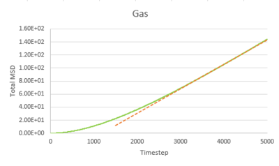
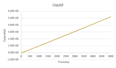
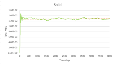
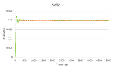
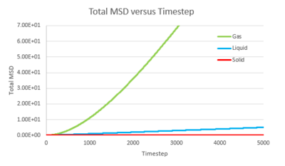
The trend of the MSD graph from our simulations is very similar to the one million atom simulations. The MSD of gas has a short non-linear region at the start then becomes linear. For liquid, the MSD increases linearly with timestep throughout. The solid has a sharp, sudden spike at the start, then decay to a constant value. The linear regions of gas and liquid corresponds to the molecule's path which resembles a random walk due to rapid collisions. in what way does it represent a random walk? The non-linear region at the start of gas MSD graph corresponds to the path of the molecule before it makes the first collision, where it moves with approximately constant velocity, the MSD is proportional to time squared.what is this region? (ballistic) This region results from the large molecule separation in gas system. The solid MSD remains constant with small oscillation after the initial collision, indicating the solid molecule remains localized with respect to the reference position over time. This is due to the ordered, close-packed structure of solid. Notice for the large system simulation, there are hardly ever oscillations around the equilibrium MSD, it makes a better approximation. As shown in the combined graph, the increase of MSD over time declines from gas to solid.Increase declines? Call it what it is! The gradient The gram is due to fewer collisions in more diffused systems leads to faster movement of molecules.

The diffusion coefficient, D, is calculated from the gradient of the linear region of the MSD graph, where the motion of molecule is purely diffusive.

Timestep = 0.002, $D=\frac{1}{6}\frac{1}{0.002}\frac{\partial ⟨r^2\left(t\right)⟩}{\partial t}$.

Table 3. Diffusion coefficient estimations (m²s^-1).

	Gas	Liquid	Solid
Our simulation	3.1947932	0.0848978	2.093525E-6
Large system simulation	3.1372520	0.0872643	1.2099417E-6

The gas has the highest diffusion coefficient and the solid has the lowest diffusion coefficient, close to zero. The value calculated from our simulation is close to the value calculated from the one million atom simulation, indicating our simulation is accurate.tick, units of diffusion coefficient??

Velocity Autocorrelation Function

Task 1 In the theoretical section at the beginning, the equation for the evolution of the position of a 1D harmonic oscillator as a function of time was given. Using this, evaluate the normalised velocity autocorrelation function for a 1D harmonic oscillator (it is analytic!):

$C\left(\tau \right)=\frac{\underset{-\mathrm{\infty }}{\overset{\mathrm{\infty }}{\int }}v\left(t\right)v(t+\tau )\mathrm{d}t}{\underset{-\mathrm{\infty }}{\overset{\mathrm{\infty }}{\int }}{v}^2\left(t\right)\mathrm{d}t}$

Be sure to show your working in your writeup. On the same graph, with x range 0 to 500, plot $C\left(\tau \right)$ with $\omega =1/2\pi$ and the VACFs from your liquid and solid simulations. What do the minima in the VACFs for the liquid and solid system represent? Discuss the origin of the differences between the liquid and solid VACFs. The harmonic oscillator VACF is very different to the Lennard Jones solid and liquid. Why is this? Attach a copy of your plot to your writeup.

The position of an 1D harmonic oscillator as a function of time is $x\left(t\right)=A\cos (\omega t+\varphi )$.

$v\left(t\right)=\frac{dx}{dt}=-A\omega \sin (\omega t+\varphi )$

$C\left(\tau \right)=\frac{\underset{-\mathrm{\infty }}{\overset{\mathrm{\infty }}{\int }}(-A\omega \sin (\omega t+\varphi ))(-A\omega \sin (\omega t+\omega \tau +\varphi ))\mathrm{d}t}{\underset{-\mathrm{\infty }}{\overset{\mathrm{\infty }}{\int }}{A}^2{\omega }^2{\sin }^2(\omega t+\varphi )\mathrm{d}t}$

$C\left(\tau \right)=\frac{\underset{-\mathrm{\infty }}{\overset{\mathrm{\infty }}{\int }}{A}^2{\omega }^2(\sin (\omega t+\varphi ))(\sin (\omega t+\varphi )\cos \left(\omega \tau \right)+\cos (\omega t+\varphi )\sin \left(\omega \tau \right))\mathrm{d}t}{\underset{-\mathrm{\infty }}{\overset{\mathrm{\infty }}{\int }}{A}^2{\omega }^2{\sin }^2(\omega t+\varphi )\mathrm{d}t}$

$C\left(\tau \right)=\frac{\underset{-\mathrm{\infty }}{\overset{\mathrm{\infty }}{\int }}{\sin }^2(\omega t+\varphi )\cos \left(\omega \tau \right)+\cos (\omega t+\varphi )\sin (\omega t+\varphi )\sin \left(\omega \tau \right)\mathrm{d}t}{\underset{-\mathrm{\infty }}{\overset{\mathrm{\infty }}{\int }}{\sin }^2(\omega t+\varphi )\mathrm{d}t}$

$C\left(\tau \right)=\frac{\underset{-\mathrm{\infty }}{\overset{\mathrm{\infty }}{\int }}{\sin }^2(\omega t+\varphi )\cos \left(\omega \tau \right)\mathrm{d}t}{\underset{-\mathrm{\infty }}{\overset{\mathrm{\infty }}{\int }}{\sin }^2(\omega t+\varphi )\mathrm{d}t}+\frac{\underset{-\mathrm{\infty }}{\overset{\mathrm{\infty }}{\int }}\cos (\omega t+\varphi )\sin (\omega t+\varphi )\sin \left(\omega \tau \right)\mathrm{d}t}{\underset{-\mathrm{\infty }}{\overset{\mathrm{\infty }}{\int }}{\sin }^2(\omega t+\varphi )\mathrm{d}t}$

$\cos (\omega t+\varphi )\sin (\omega t+\varphi )\sin \left(\omega \tau \right)$ is an odd function. Its integrate over $-\mathrm{\infty }$ to $\mathrm{\infty }$ is zero.

Therefore, $C\left(\tau \right)=\cos \left(\omega \tau \right)$ for 1D harmonic oscillator.

With $\omega =\frac{1}{2\pi }$, $C\left(\tau \right)=\cos \left(\frac{\tau }{2\pi }\right)$.tick, more generally w.T

Figure 15:Total VACF versus Timestep.

The VACF of all three phases start from their maximum value then decay to o overtime. Gas phase decays slowest. That is because gas molecules are very diffuse, there are very few collisions between molecules to slow them down. Therefore, the difference between velocity at time $t+\tau$ to that at time $t$. The velocity took a long time to become independent. Liquid VACF reaches zero quickly, as molecules are more packed and more collisions to slow down the molecule. Solid molecule collides with neighboring molecules at first then oscillates around its lattice position. Its VACF decays to zero very quickly. The minima in the VACFs for the liquid and solid system represent the back scattering motion. As for the 1D harmonic oscillator, its VACF shows a periodicity. This is because the velocity of it also has a periodicity, it increases then decreases periodically overtime.what do the minima mean?

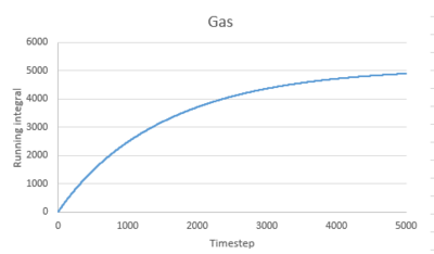
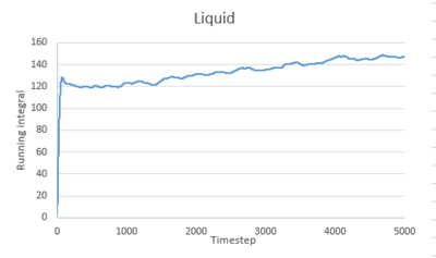
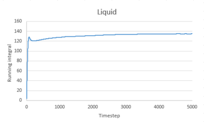
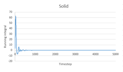
Task 2 Use the trapezium rule to approximate the integral under the velocity autocorrelation function for the solid, liquid, and gas, and use these values to estimate $D$ in each case. You should make a plot of the running integral in each case. Are they as you expect? Repeat this procedure for the VACF data that you were given from the one million atom simulations. What do you think is the largest source of error in your estimates of D from the VACF?

Table 4. Running integral of VACF.

	Our simulation	One million atom simulation
Gas	Running integral under VACF of gas.	Running integral under VACF of gas for larger systems.
Liquid	Running integral under VACF of liquid.	Running integral under VACF of liquid for larger systems.
Solid	Running integral under VACF of solid.	Running integral under VACF of solid for larger systems.

Table 5. Diffusion coefficient estimations from VACF(m²s^-1).

	Gas	Liquid	Solid
Our simulation	3.294631407	0.097880239	0.000405854
Large system simulation	3.268510202	0.090092396	4.54794E-05

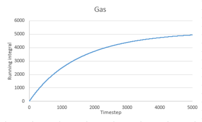
The running integral of VACF for gas increases quickly at the start then increases slowly to level off. For liquid and solid, there is a sharp spike at the start then the graph levels off.This is consistent to what VACF graphs showed before. The gas molecule velocity becomes uncorrelated slowest. For liquid and gas, the VACF quickly reach zero and the integral remain constant.

The diffusion coefficients estimated from the integral of VACF are close to that estimated from the MSD graph for gas and liquid. However, for solid, the estimations are different. There are several sources of error contribute to this. Firstly, we used trapezium rule to estimate the integral, which is a poor method. I wouldn't call it poor! 0.002 was used as timestep. smaller timestep could be used to give better approximation of integral. Secondly, not enough data was obtained. The VACF was only recorded for 10 seconds. This leads to inaccurate estimation of D.

Conclusion

In this experiment, we preformed computer molecule dynamic simulation. Gram!! There are a number of things wrong with this sentence! It gives us an idea of how computer simulation is generated and how different set-ups such as timestep influence the results.really vague... The results obtained gives information of molecule movement over time at each timestep. We also investigated how different thermodynamic properties changes with different phases under different conditions and how the results obtained correlated to structural properties of different phases. Although the simulations done in this experiment ignore many other factors that may contribute to molecular motion, it still provide gram a resonable picture of dynamic changes of molecules that is valuable in investigations about molecule behaviors.gram! and really vague... molecular behaviours? Specifically the dynamic and diffuse properties of phase...