Jt3818

Exercise 1

On a potential energy surface diagram, how is the transition state mathematically defined? How can the transition state be identified, and how can it be distinguished from a local minimum of the potential energy surface?

Transition state (TS) is a saddle point on the potential energy surface. That means that the gradient is zero $\mathrm{\nabla }F=0$ but the point is neither minimum nor maximum. The second partial derivative test can be used to identify a saddle point. Let $f(x,y)$ be a function of x and y, then $D=f_{xx}(x,y)f_{yy}(x,y)-f_{xy}^2$:

1. If $D(a,b)>0$ and $f_{xx}(a,b)>0$, then a point (a,b) is a local minimum

2. If $D(a,b)>0$ and $f_{xx}(a,b)<0$, then a point (a,b) is a local maximum

3. If $D(a,b)<0$ then a point (a,b) is a saddle point

4. If $D(a,b)=0$, then the test is inconclusive.

1. a
2. 2

For the multivariable functions, the test is defined in terms of the eigenvalues of the Hessian matrix.

1. If the Hessian is positive definite at a, then f has a local minimum at a.

2. If the Hessian is negative definite at a, then f has a local maximum at a.

3. If the Hessian has both positive and negative eigenvalues then a is a saddle point of f

Otherwise, the test is inconclusive.

Therefore, a local minimum can be distinguished from a saddle point using the second partial derivative test.

Trajectories from r₁ = r₂: locating the transition state

To locate the TS, both internuclear distances were taken to be equal and the momenta were set to zero because the TS is expected to be centrosymmetrical (the reaction entalpy is zero). Since the TS is a saddle point, there are no forces acting on the nuclei: $F=-\mathrm{\nabla }V=0$ where V is the potential energy. The nuclear separations were changed until the forces were close to zero. The separation in the TS was found to be r₁ = 90.8 ppm to 3 significant figures. The magnitude of the forces were 0.004 kJ/pm mol. Figure 1 which shows the countour plot with the TS designated with a cross and the variation of the positions of the atoms which is essentially constant.

• 
  Figure 1 a) PES for r_AB = r_BC =90.8 ppm
• 
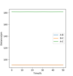  b) Distance vs Time plot for r_AB = r_BC =90.8 ppm

Calculating the reaction paths

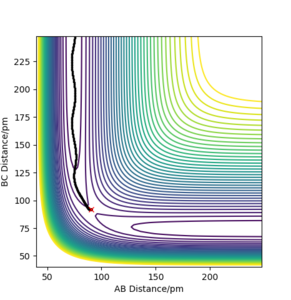
The minimum energy path (MEP) was generated starting from the point slightly displaced from the TS. It can be thought as a displacement from the unstable equilibtrium of the PES downhill in direction of the steepest descent. The traced path is shown in Figure 2a, where the path is shown as a solid black line. It is evident also from the plot of the nuclei position against the time (Figure 2b), that there were no molecular vibrations and that atoms were smoothly changing their positions.

• 
  Figure 2 a) PES contour plot of the MEP calculation for r_AB = 91.8 ppm, r_BC =90.8 ppm, p_AB = p_BC = 0
• 
  b) Internuclear distances vs time for the system described in Figure 2a

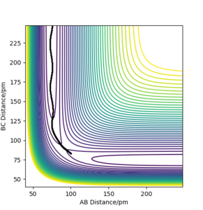
On the other hand, when the dynamics simulation was run, the formed H₂ molecule was vibrating thus the path depicting the nuclei motion in Figure 3a is more curvy due to the molecular vibrations. When the internuclear distances r_AB, r_BC were swapped, the particles were moving downhill in the direction to the second valley (Figure 3b, the trajectories are mirror images with respect to the diagonal of the plot). Then, the values of the positions and momenta from the last data points (obtained from the exported data) and the calculated trajectory (Figure 3c) is analogous to the one depicted by Figure 3b. Thus, the calculation is consistent as it gives a very similar trajectory for the reverse process.

• 
  Figure 3 a) PES contour plot for r_AB = 91.8 ppm, r_BC =90.8 ppm, p_AB = p_BC = 0
• 
  b) PES contour plot for r_AB = 90.8 ppm, r_BC =91.8 ppm, p_AB = p_BC = 0
• 
  c) PES contour plot for r_AB = 74 ppm, r_BC = 353 ppm, p_AB = 3.21 g·mol⁻¹·pm·fs⁻¹, p_AB = 5.10 g·mol⁻¹·pm·fs⁻¹