
Jb40608
BCl3
In this section of the module I created and optimised a molecule of BCl3 to obtain information about the molecule. A precursor model of the molecule was created in Gaussview, then optimised in shape, using the FOPT calculation type, the RB3LYP calculation method, and the 3-21G basis set. The output was saved in a gaussian log file (.log). The information about the calculation used and information gained about the molecule are summarised below.
| Caluculation information | Value |
| file type | .log |
| calculation type | FOPT |
| calculation method | RB3LYT |
| basis set | 3-21G |
| calculation time | 23.0 sec |
| Molecule information | Value |
| final energy | -1398.8044943 A.U. |
| dipole moment | 0 Debeye |
| point group | D3H |
BCl3 |
Creating and optimising a small molecule
Here I created a small molecule in gaussview and used previously used methods to optimised it and obtain information about its electronic and nuclear structure.
I decided investigate CO2 in this small molecule section, and optimised it via the B31LYP and the 3-21G method. The information about the optimised molecule was taken from the log file and recorded in the table below.
In the .log file the atoms that comprise the molecule are given identifiers - they have been removed here. However in the bond angles section the angle A1 refers the C=O bond, and the A2 angle refers to the C=O' angle.
N.B. O' is just to distinguish between the two oxygens.
| Properties | Values | ||||
| xyz coridinates (Angstroms) | C - 0.000000, 0.000000, 0.000000 | O - 0.000000, 0.000000, 1.258400 | O' - 0.000000, 0.000000, -1.258400 | ||
| Bond Lengths(C=O) / Angstroms | 1.258400 | ||||
| Bond angles | Bond descriptor | Definition | Value | Derivative information | |
| A1 | L(2,1,3,-1,-1) | 180.0 | estimate D2E/DX2 | ||
| A2 | L(2,1,3,-2,-2) | 180.0 | estimate D2E/DX2 | ||
| Calculation method | optimisation using the B3LYP calculation | ||||
| Basis set | B-31G | ||||
| Point Group | D*8 | ||||
| Final Energy (a.u.) | -187.5236 | ||||
| dipole moment (Debye | 0.000 | ||||
| Time taken for calculation (Seconds) | 13.0 | ||||
CO2 |
Vibrational analysis
Here I took the optimised structure of BH3 and used gaussview to calculate the vibrations of the molecule. I did this by changing the input file to
# freq b3lyp/3-21g geom=connectivity pop=(full,nbo)

BH3  frequency

0 1
 B
 H                  1              B1
etc.
The output was saved, and the vibrations analysed.
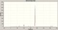
There were 6 vibrations, listed in the table below. The predicted total spectrum is posted to the right.

| Vibration number | Vibration visualisation | frequency | intensity | point group |
| 1 | 
|
1117.58 | 95.5092 | a2 |
| 2 | 
|
1186.21 | 11.318 | e |
| 3 | 
|
1186.21 | 11.3204 | a2 |
| 4 | 
|
2687.5 | 0 | a1 |
| 5 |  asymmetric stretch from right to left asymmetric stretch from right to left
|
2834.38 | 102.206 | e |
| 6 |  all 3 move together in and out of the page all 3 move together in and out of the page
|
2834.38 | 102.119 | e |
As we can see from the spectrum only 3 peaks appear, despite 6 being predicted. With vibrations 1 and 2 the vibrations are close enough in frequency to be seen together, while 5 and 6 have exactly the same point group and also absorb at exactly the same frequency so only 1 peak is seen. Vibration 1 still is visible. However with vibration 4 there is no net displacement, making it IR invisible, hence the non absorbance.
BCl3 |
Molecular orbitals
From the frequency out file I used gaussview to construct the molecular orbitals, summerised in the table below. I also contructed my own MO diagram, displayed to the right of it.

- MO visualisation
-
 MO 1, relative energy: -6.552
 -
 MO 2 relative energy: -0.586
 -
 MO 3 relative energy: -0.439
 -
 MO 4 (HOMO) relative energy: -0.439
 -
 MO 5 (LUMO) relative energy: -0.208


Comparing the 2 we can see a good correlation between the 2, with no discrepancies seen.
Cis and Trans isomerism in organometallic complexes
In this section of the module I optimised the structure of 2 molybenum isomers (cis and trans) by serval steps. To do this I used the scan service provided by the college, as the calcualtions were sufficiently labour intensive to overheat the laptops provided for this course. To do this I put the calculations I wanted doing into gaussview, then saved the relevant gaussian input file without running it on the laptop. I then located the relevant gaussian input file and submitted it to the scan service.
The isomers I was investigating were the cis and trans isomers of Mo(CO)4(P(CH3)3)2.
Initially I constructed the 2 isomers in gaussview, using the relative molecule fragments before beginning to optimise the molecules.
The initial calculation was a B3LYP method optimisation, using the LAN2LMB basis set., with the additional commands being "opt=loose".
# opt=loose b3lyp/lanl2mb geom=connectivity

james_cisMo_opt

0 1
 Mo                0        -2.82051268      0.59829059      0.00000000
etc.
This was tested on the laptop for 5 minuetes before submitting to scan; if the calculation completed within this time there was a problem with the input file, and had to be remeedied. No problems were encountered and these were submitted to scan overnight.
Once both optimisations had finished the log files of both were downloaded, and a new input attached, using a more accurate basis set, and electronic convergance data added.
# opt b3lyp/lanl2dz geom=connectivity int=ultrafine scf=conver=9

james_cisMoFurther_opt

0 1
 Mo
 C                  1              B1
etc.
The finalised geometries were downloaded, and their D-space identifiers are cis:http://hdl.handle.net/10042/to-1377, trans: http://hdl.handle.net/10042/to-1389.
The final structures:
cis optimised |
Optimised cis structure
trans optimised |
| Isomer | energy (a.u.) |
| cis | -733.3602 |
| trans | -733.3573 |
When we compare the energies of the 2 isomers we see that both are very similar in energy, but the trans isomer is slightly more stable (by about 7.614kJ/mol). In order to change the order of the cis and trans isomers you could use several methods: you could use bidentate ligands which only permit certain geometries to be obtained, or you could have substituients that could favourably interact - e.g. hydrogen bonding.
From literature [1] I was able to gain the experimentally determined geometeries. However gaussview has recorded them in a different orientation and distance units to the literature values, making comparision unsuitable.
Once these had been obtained I used the optimised structures to predict the IR, using the methods described in the vibrational analysis section. The results are summerised in the table below.
- IR graphs
-
 Predicted cis isomer IR
 -
 Predicted trans isomer IR


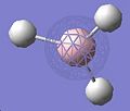
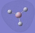
The quantum Nature of ammonia
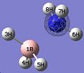
In this section I shall be using the methods I have already learned to understand the quantum nature of ammonia. This 'quantum nature' of ammonia refers to the fact that the lone pair can 'tunnel' from one side to the other, changing the geometry of the molecule as it does so.
Initially I looked at the normal geometry of ammonia, by constructing and optimising a NH3 molecule within gaussview, using a B3LYP calculation method and a B-21G method.
I then manually altered the bond length of one of the N - H bonds (to 1.01Å, from 1) , and reoptimised the molecule (telling it to ignore symmetry whilst doing so) to see what the resultant point group would be.
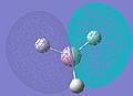
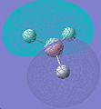
Using a preprepared molecule I examined what would be the intermediate geommetry of the transition; this preprepared molecule had a dummy atom locking it into position.
| Value | |||
| Property | Ground state | Broken symmetry | Transition state |
| Energy / a.u. | -56.229126 | -56.229128 | -56.42664911 |
| Dipole Moment / Debye | 1 .8678 | 1 .8678 | 0.0000 |
| Point Group | C3V | C1 | D3H |
Examining the 3 different molecules obtained via these calculations there is very little discernable difference (apart from the diffrence in bond length which I applied) between the C3V and the C1 geometries, but examining the bond angles showed there to be slight differences - the C1 point group one had a slightly bigger bond angle. However a difference in energy was seen as well. Also the time taken to gain each optimised structure was different - C3V took 16 seconds, C1 took 32 seconds and D3H took 1 minute 47 seconds.
If we examine the energies of the diffrent geometries we can see that they become more negative as the molecule breaks from its regular structure to the planar structure. This is important since it shows that there is a energy barrier to be crossed in this transition from one state to another - it requires an input of energy. I then used a more accurate method for determining the energies and geometries of the starting and transition states - the MP2 method, using the 6-311+G(d,p) basis set. The resulting energy difference:| State transition | difference in Energy (kJ) |
| Ground state/Breaking from symmetry | 0.0052509 |
| Breaking from symmetry/transition state | 518.579 |
| State transition | difference in Energy (kJ) |
| Ground state/transition state | 80.9563 |
| State | Jmol | |||
| Ground state |
| |||
| transition state |
|
Mini Project
For this section I decided to investigate what has been touted as the future of hydrogen fuel - a borone/ammonia molecule. I decided to investigate the molecule to examine its stability, and its suitability as a fuel. It has been decribed as the future due to its high hydrogen content, and its stability at room temperature. Key to this molecules application as a fuel is the fact that it has a strong N-B bond, favouring dissociation of H opposed to the breaking of this bond.
Firstly, I shall investigate the structure of the proposed fuel, then I shall move onto determining the orbital set up and the bonding present in the molecule.

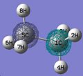
The structure of the borane/ammonia molecule was first constructed in chemdraw, in the eclipsed formation, before being saved as a gaussian input and opened with gaussview. The molecules geometry was obtained with a DFT, B3LYP, 3,21G optimisation. The output file was opened, and the intermediate geometries examined. The optimisation showed that the staggered conformation of the molecule was the most stable.
| Structure |
|
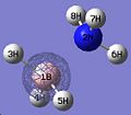
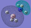
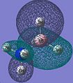
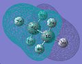
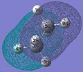
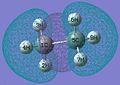
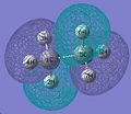
Thus, the optimised geometry was optained. From this file I proceeded to run a frequency calculation on the molecule, to see the energy distribution between the MOs. This was compared to a MO diagram constructed by myself, displayed below, to the right. I set the isovalues to 0.02 to examine the orbitals, changing the value of it if I was uncertain of the contribution of specific atoms. There was good equivalance.

- visual reprentations of the MOs of ammonia borane
-
 MO 1
MO 1 -
 MO 2
MO 2 -
 MO 3
MO 3 -
 MO 4 - equivalent in energy to 5
 -
 MO 5 - equivalent in energy to 4
 -
 MO 6
MO 6 -
 MO 7
MO 7 -
 MO 8 - equivalent in energy to 9
 -
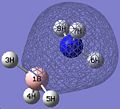
 MO 9, HOMO - equivalent in energy to 8
 -
 MO 10, LUMO


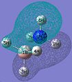
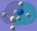
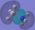
From this we can see that there is sigma and pi bonding between the two halfs of the molecule (interpreted as electron density between the 2 fragments, and electron density parallel but not laying directly along the bond respectively), though seemingly unstable orbital formations are also occupied. This can be explained by the fact that the electron density is not equal between the two fragments, so this could be a representation of more ionic bonds.
Closer examination of the MO diagrams shows high electron density between the N and the B, and low electron density around the hydrogens, with the density delocalised so that it is not directly lying between the N and the B in several MO conformations. This supports the idea that the N-B bond is stronger, and H dissociation is more likely.
Comparision with a equivalent molecule
If we then examine ethane (see below), we see the same general electron distribution across the molecule, though with the ammonia borane molecule the electron density is usally focused on one of the 2 fragments. However the predicted MO energy levels are more stable - lowering energy.
- Molecular orbitals of ethane
-
 MO 1
MO 1 -
MO 2
-
 MO 3
MO 3 -
 MO 4
MO 4 -
 MO 5
MO 5 -
 MO 6
MO 6 -
 MO 7
MO 7 -
 MO 8
MO 8 -
 MO 9
MO 9


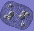
|
| The unit cell of solid ammonia borane. |
It has been reported that ammonia borane has a much higher boiling point compared to its isoelectronic equivalent, ethane. In various literature reports[2] this has been attributed to dihydrogen bonding - interactions between the hydrogens on the N with hydrogens on the B.
This can be explained if we look at the distribution of charge on the molecule - the hydrogens on the borane fragment are negative, whilst the hydrogens on the nitrogen fragment are positive. This allows for the formation of a regular crystal structure. This form of bonding, compared with only Van der Waals interactions present in ethane, contribute to the overall stability of the molecule.
Ethane obviously cannot form this dihydrogen bonding, since there is no net differnce in charge between any of the hydrogens, all being equally polarised by the C-H bond, as opposed to the different elctronegativites of the centeral atoms of the fragments in ammonia borane.
Now that we have identified several key structural features about ammonia borane we can discuss its suitability as a hydrogen resevoir.
When we look at the MOs of ethane and ammonia borane we can see that at a isovalue of 0.02 the electron density on ammonia borane often does not extend to some hydrogens, that when we look at ethane have electron density on, or have some shielding from the orbitals. This is particularly appreciable in the HOMO - most of the elctron density is focused on the borane fragment, leaving little on the ammonia fragment. It also left 1 hydrogen totally without elctron density, which leaves it succeptable to nucleophilic attack.
This supports the idea the the B-N bond is much less likely to be broken than the formation of H2 - One of the main ideas as to why this would make a good hydrogen resevoir. Various other features of the molecule taken from the litrature show tha the main methods of extracting the hydrogen were heating the solid stat to ~ 100°C and using a BH3 catalyst. Both of these make the use of this substance favourable, since it would not be difficult to produce the conditions required for hydrogen to be produced - though controlling the rate of production of hydrogen would be difficult using a catalyst; you could end up with the fuel tank expanding and rupturing if left unused for too long!

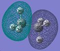
|
| Charge distribution across the molecule. Red is negative, green is positive.
The window within this shows the variation of colour with charge |
The fact that it can form a solid state matrix is also good for its application as a fuel source - it would not require special reinforced containers as with hydrogen gas, making it easier to handle and transport. Also this increases the density of hydrogen without the need for excessive conditions (e.g. high pressures), a important consideration when you want to maximise the space for people or things to be transported.