1da-workshops-2013

Introduction to Chemical Programming Workshop 2013/14

This workshop contains a series of exercises in data processing using MATLAB. The purpose of this exercise is not to provide a detailed lesson in a particular piece of software, but to introduce some of the ways in which computers can be used to automate the majority of the "heavy lifting" when it comes to analysing data that you might produce in your experiments. The programming techniques that we will introduce are common to very many, if not all, languages, and the mathematical tools provided by MATLAB are also available in many other free and commercial packages. Some links to other similar software packages will be provided at the end of the article for those interested in expanding their knowledge.

If you have a question, or find a mistake, please check the discussion page. We encourage you to use that page to ask any questions that you might have, or to see if your classmates have similar queries.

You will find that this script occasionally makes reference to the other wiki. Where this happens, it is to provide a little background information on a relevant concept, or to serve as a refresher of a concept which you may not have seen in a while. As usual, you should be careful not to get bogged down. Mathematical and scientific articles on Wikipedia can become extremely technical very quickly!

Preamble: Introduction to Programming in MATLAB

Starting MATLAB

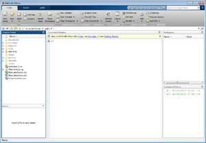
MATLAB can be found on the chemistry department computers on the start menu as MATLAB R2013a. If you wish to install a copy on your own computer for your personal use, you can do so by following the instructions here (select 'Matlab' from the table of options).

After starting the program you will see the MATLAB Desktop (shown in figure 1). This window contains 4 important panes: Current Folder, on the left; Command Window, in the centre; Workspace, in the top right, and Command History, in the bottom right. The Current Folder pane is a convenient way to browse the local filesystem from within MATLAB. For these exercises, you should navigate to a suitable folder on your computer and create a folder in which to store your work by right-clicking in the Current Folder pane. A folder called MATLAB in the directory \\ic.ac.uk\homes\your college username would be appropriate. The Workspace lists all of the variables which are currently defined. We will define what we mean by a variable in a moment. The Command Window is used to type commands, and is also used to display the results of certain commands. The Command History keeps a record of the commands that MATLAB has received. Unless you have used MATLAB before, this will be blank. You will notice that one of the panes is highlighted and bordered in dark blue. This denotes the active pane, and is usually the last pane that was clicked by the mouse. Try clicking the four panes described above, and see what happens.	Figure 1: The MATLAB desktop
Click on the Command Window to make it active, then press F1. A small help window will open. In the bottom left is a link which reads "Open Help Browser", which you should click. The MATLAB documentation will then open (figure 2). This documentation contains the details of every MATLAB command, as well as lots of information about the interface. Figure 3, for example, shows the documentation entry for the MATLAB desktop screen itself, which we saw above. There will be points in this script at which you will be told which MATLAB commands to use, but not how to use them. At such times, you should look up the commands in this help window.	Figure 2: MATLAB help browser Figure 3: the documentation for the MATLAB desktop

Some basic programming concepts

In this section, we will introduce the basic ideas behind storing and manipulating data in MATLAB.

Variables

Scalar variables

Most programming exercises boil down to the manipulation of variables, which are the means by which we have the computer store information. Try typing the following code at the prompt, then pressing return.

a=6

a is a variable, with the value 6. MATLAB will provide you with some output, which will look a little like that in figure 4.

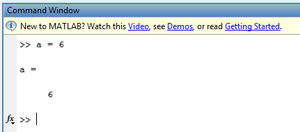
Figure 4: the result of the command a=6

This output is often not very useful, and you can suppress it by ending your command with a semi-colon (;). Try running the command:

b=7;

You will notice that MATLAB remains completely silent, but look at the Workspace pane on the right hand side of your screen (figure 5). Both variables that we have defined are listed here, along with their values

Figure 5: Workspace pane after two variables have been defined

. This pane can be used to see which variables have been defined, and to edit their values. Try double clicking one of the variables names and see what happens.

You can display the value of a variable at any time by simply typing its name. For example, the command a displays the same output as shown in figure 4.

Now try the commands a*b, a+b, a/b, and a-b. You should find that they all behave as you would expect, and that you can use MATLAB as a somewhat overpowered calculator.

Matrix Variables

One of MATLAB's great strengths is the ease with which it can perform linear algebra operations. As well as scalar variables, we can define matrices and operate on them. Define the matrix c, using the following command:

c = [1 2 3; 4 5 6; 7 8 9;]

The spaces separate columns of the matrix, while semi-colons separate rows. By convention, a matrix with $n$ rows and $m$ columns is called an $n\times m$ matrix. The matrix that we have entered is

$\left(\begin{array}{ccc}1& 2& 3\\ 4& 5& 6\\ 7& 8& 9\\ \end{array}\right)$,

which is a $3\times 3$ matrix. Once again, you should try double clicking on the variable c in the Workspace pane on the right hand side. You will find that you are able to edit this matrix if you wish.

Figure 6: suppressing output with the colon

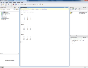
Suppose we want to square every element of our matrix. This is called an element-wise operation, since it operates on each element of the matrix in turn. Element-wise operations are denoted by placing a full-stop before the operator.

To square the matrix, we use the command c.^2. Compare this to the output of the command c^2. This second command computes the square of the matrix itself (i.e. c*c). This is not the same as multiplying each element by itself, as figure 6 shows.

Matrix variables are particularly useful for us, since we can use them to store time series. Imagine that we have a piece of lab equipment that takes measurements automatically at specified intervals, and stores these data in a file that we can read with MATLAB. We can store the time of the measurement and the value measured in two vectors. If we make $N$ measurements, both of these vectors will be of size $N\times 1$.

Accessing elements of matrices

We can access particular elements of a matrix using index notation. Consider the matrix c, as defined above. To access the element in the second row of the second column, we use the syntax c(2,2). For the third column of the first row, we use c(1,3) (we index the row first, and then the column). You should experiment with this, and ensure that different indices give the results you expect.

Try to calculate the trace of the matrix c: this is the sum of the diagonal elements, from top-left to bottom-right.

Conditionals

For the computer to be of any use to us, it must be able to make simple decisions. We achieve this with conditional statements:

if some test is passed

do X

otherwise

do Y

As a simple example, suppose we want to simulate the flipping of a coin. MATLAB provides a function, randsample which will pick a random integer for us from a specific range.

The command randsample(n, k) will give us $k$ random integers, from the range $[1,n]$. If we use the command randsample(4, 2) we will get two random integers, which will either be 1, 2, 3, or 4.

To simulate our coin flipping, we can use the command coin = randsample(2,1);, which will return a single random value, either 1 or 2, and store it in the variable coin. We will then say that a value of 1 corresponds to heads, and a value of 2 corresponds to tails. The if command that we must use takes the following form:

if coin == 1

'Heads'

else

'Tails'

end

Once an if command begins, MATLAB will not try to run the command until it encounters an end command. This command can therefore easily be typed over 5 lines, as shown here (and in fact, this is required).

Note the double equals sign used on the first line! The statement coin = 1 means "Store the value 1 in the variable coin". This is not what we want at all! Instead, we use coin == 1, which means "Compare the value of the variable coin and the number 1. If they are the same, this statement is true. Otherwise, this statement is false". To use more precise terminology, the single equals sign ($=$) assigns the value on the right hand side to the variable on the left hand side, while the double equals sign ($==$) checks for the equality of the values on each side.

Loops

Loops allow us to perform the same task many times. To consider a contrived example, imagine that we have a column vector, X, and that we want to print every element of this vector and its square. We first define the vector X with the command:

X = [1 2 3 4 5];

To act on every element in our vector, we use a for loop.

for i = 1:5

i

X(i)

X(i)^2

end

Like the if statement, once a for command begins, MATLAB will not execute any instructions until it reaches the corresponding end command. The first line is more easily understood if we read it from right to left.

• 1:5 instructs MATLAB to create a 1x5 matrix, whose elements are 1, 2, 3, 4, and 5. In fact, the command 1:5 has the same result as the command [1 2 3 4 5];, and is a convenient shorthand.
• i = assigns this matrix to the variable i. This variable is often referred to as a loop counter.
• for tells MATLAB to read the instructions on the following lines (until it reaches the end command), and to execute them for every element of the variable i.

This for loop will run fives times, with i equal to 1, 2, 3, 4 and then 5. In each case, it will show the value of i (i), show the value of X at that position (X(i)), and finally show that value squared (X(i)^2).

The size Function

We might not know exactly how large the matrix X is. Alternatively, we might want to write a script which we can use over and over again, on many differently sized matrices. If this is the case, our for loop may not work; after all, at the moment it only counts to five. If we have a matrix with ten columns, we will only see half of our data. MATLAB provides a function, size, which allows our scrits to find out how large a particular variable is.

Try the command s = size(X). You will see that the answer is itself a matrix, with two columns. The first column, s(1), stores the number of rows, while the second, s(2), stores the number of columns. You should try the loop code above again, but this time using the size function so that it could work with a matrix of any size.

Array Slicing/Reshaping

Sometimes, having defined an array, we may want to throw some of it away. Consider, for example, that we have loaded an array of size 1000x1, but that we only want to keep the data from row 50 onwards. It may be that this is experimental data, and that the first 49 measurements were taken incorrectly. We'll call this first array raw_data, and we'll define a second array called valid_data to contain the information we keep. We can use an 'array slice' (sometimes called array reshaping) to get rid of some of our data. In this case, we want our new array to contain only those elements of the old array from row 50 or above.

valid_data = raw_data(50:end)

The 50:end in the brackets indicates that we want to keep only those elements between row 50 and the end of the array. If we wanted only rows 50-70, we could use the command:

valid_data = raw_data(50:70)

This also works on matrices. If we have a 4x5 matrix, X,

X = [1 2 3 4 5; 6 7 8 9 10; 11 12 13 14 15; 16 17 18 19 20]

we can extract a variety of 3x3 matrices. For example:

s = X(3:end, 3:end)

Figure 7: extracting a 3x3 matrix from a larger one

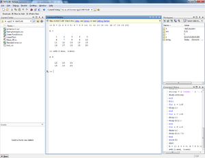
To get the new matrix s, we take only those data from X which have both row and column indices >= 3, and end up with figure 7.

Array slicing is extremely useful!

Functions

Functions are a way of grouping together statements to make their use simpler. Defining your own functions is a little like writing your own MATLAB commands.

Consider the following situation: you have a large amount of experimental data that is extremely noisy, stored in the variable noisy_data. You know a complicated sequence of MATLAB commands which will clean up this data. To avoid having to type these commands every time you want to clean up data of this type, we can define a function, which we shall call my_cleanup_function. Extracting the useful data is then as simple as typing the statement:

clean_data = my_cleanup_function(noisy_data)

You can keep your function forever, and never again have to worry about unclean data (this is, unfortunately, not how reality works).

Imagine that we have a friend who knows very little about how to use MATLAB. Our friend has managed to define a matrix, X, and wants to multiply every element by 7, before adding 4. He or she has agreed to pay us a great deal of money if we can send him/her some code which will do this for them. To do it, and to keep things nice and simple for our friend, we will write a function to do this operation. Since we lack imagination, we shall call it TimesSevenThenAddFour.

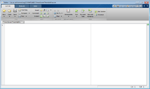
MATLAB doesn't allow us to define functions in the Command Window; we have to do this using a text editor. Make sure that your Current Folder pane is set to browse the MATLAB folder that you created earlier, then right click in the Current Folder pane. Select New file → Script. You'll be prompted to choose a name for this file, which will be TimesSevenThenAddFour.m Once you have done this, you should see the file in the Current Folder pane. To open the file in the editor (figure 8), double click it.

Figure 8: the MATLAB script editor

We can now write our function. The first line should be:

function ret = TimesSevenThenAddFour(x)

The first part, function, simply tells MATLAB that we are making a new function.

The second part of the command, ret = , sets up the return value of the function: this is the value that our friend will get back when he uses our function. For example, in the size function, the return value is the size of the given matrix. Whatever value we assign to ret in our function is the value our friend will get back.

Finally, TimesSevenThenAddFour(x) tells MATLAB the name of our function, and also sets up the argument list. This is the list of variables which our friend will need to pass to our function in order for it to work properly. In this simple case, we only need a single variable: the matrix that our friend wants us to transform.

On the next line of our function, we need to perform the actual operations. In our case, this is simple:

ret = x*7 + 4;

Note that we use the semi-colon to suppress the output. Our friend doesn't want to be bothered by our function printing out everything that it does.

Finally, we end our function by putting end on the next line. Our whole function is:

function ret = TimesSevenThenAddFour(x)

ret = x*7 + 4

end

Save this file in the editor, then close it. Returning to the Command Window pane, we can now define some test data: test = 10:20. Try calling our new function with the command TimesSevenThenAddFour(test).

Simple plotting

We can plot data in MATLAB using the plot command. In its simplest form, this command takes two arguments: a matrix of x values, and a matrix of y values. In the last section, we wrote a function called TimesSevenThenAddFour, which we will use again here.

Create some x values from 0 to 50: x = 0:50. Now use our function to create corresponding y values, y = TimesSevenThenAddFour(x). Use the plot function, as described above, to plot the y and x data.

Use the panning and zooming tools in the plot window to convince yourself that the line plotted has the equation that you would expect it to, then use the built-in MATLAB help to find out how to label the x and y axes (you will need to look at the documentation for the plot command, and then look at the examples section).

To plot multiple functions on the same graph, we simply keep giving argument to plot. We can give as many pairs of x and y data as we like. As an example, try the following:

x = 0:0.1:10;

plot(x, x, x, sin(x))

Which two functions have been plotted?

Tidying up (and loose ends)

Before we start to analyse any data, it is helpful to tidy up the variables that we have created in this introduction. The command clear all will erase any variable currently defined, while clc will clear the Command Window.

You should also use the command format long. This will cause MATLAB to print values to a higher precision than is normally used.

Finally, where you have been provided with semi-completed code, you may find comments. Comments are used to make notes in the code both for yourself, and for other programmers who may see your work. MATLAB will ignore them completely. We denote comments by a % sign. When MATLAB encounters this, it will ignore the rest of that line.

%this line contains only a comment, and MATLAB will do nothing

a=7; %this comment comes after the command. MATLAB will assign the variable as normal

%this won't work though, because the comment is *everything* after the % b=6;

Task 1: Estimating Experimental Errors

Experimental values always have an associated error. You should be cautious of reported quantities which do not state what this error is! When reading the literature, you will come across statements like "The measured temperature was $$\begin{gathered} 204.5\pm 0.2 \\ \mathrm{K} \end{gathered}$$."

This means that the actual temperature lies somewhere between $$\begin{gathered} 204.3 \\ \mathrm{K} \end{gathered}$$ and $$\begin{gathered} 204.7 \\ \mathrm{K} \end{gathered}$$. If we take a second measurement and get the value $$\begin{gathered} 204.8\pm 0.4 \\ \mathrm{K} \end{gathered}$$, we can't really tell if the temperature has changed. We say that the two temperatures are the same within error.

If we assume that all of our equipment works perfectly, is properly calibrated, and is used correctly (in other words, if we eliminate systematic error), then the uncertainty in our measurements comes from random error.

In such cases, we take the average of repeated measurements to minimise the impact of the random error. To assess the quality of our data, we require three quantities.

If we take $N$ measurements, which we call $x_1,x_2,\dots ,x_i,\dots ,x_N$, these three quantities are:

• the mean

$\overline{x}=\frac{1}{N}\sum _{i=0}^N{x}_i$

• the standard deviation, which measures the distribution of the measured values about the mean.

$s_N=\sqrt{\frac{1}{N-1}\sum _{i=0}^N{(x_i-\overline{x})}^2}$

• the standard error of the mean

${\mathrm{S}\mathrm{E}}_{\overline{x}}=\frac{s_N}{\sqrt{N}}$

An explanation of the second two expressions, and why the third expression is "the error in the mean", is beyond the scope of this workshop. If you are interested, you should either use your favourite search engine, your favourite maths or statistics textbook, or consult the further information at the bottom of this page.

Simple Statistics in MATLAB

In this section, we will determine the mean and standard error in several large sets of data. This data is provided in a comma-separated values, or CSV, file. Columns are separated by commas, and new rows are indicated by a new line. MATLAB provides a function to read data from such files, named csvread.

The data for this exercise is stored in the file TimeSeries1.csv. You must make sure that this filename is listed in the Current Folder pane. Load the data into a variable called raw:

raw = csvread('TimeSeries1.csv');

You can view this data in a spreadsheet-like format by double-clicking the raw variable in the Workspace pane. This is time series data: the first column contains the time at which the measurement was taken, while the remaining columns contain the values that were recorded on the various experimental runs. It will be helpful for our purposes to separate this into two variables: a vector of times, and a matrix of recorded values. We can do this with the array slicing technique that we encountered before.

First, split the first column of the data off to form the times variable.

times = raw(:,1);

The colon in the first index tells MATLAB that we want to keep every row, while the second index specifies that we want to keep only column 1.

Then create a variable measurements to store the experimental values.

measurements = raw(:,2:end);

Use the Workspace pane to check that these new variables have the dimensions you would expect.

The MATLAB function mean can then be applied to our measurements variable to determine the mean value of each measurement. The documentation tells us that mean accepts either vectors or matrices. If we pass a vector, like times, then mean returns a single value. If we pass a matrix, like data, then mean will determine the mean for each column of the matrix, and return a row vector containing these mean values. std returns the standard deviation and acts in a similar fashion.

$\left(\begin{array}{c}{x}_1\\ x_2\\ \dots \\ x_i\\ \dots \\ x_N\end{array}\right)⟼\overline{x}$

$\left(\begin{array}{ccc}{a}_1& & z_1\\ a_2& & z_2\\ \dots & & \dots \\ a_i& & z_i\\ \dots & & \dots \\ a_N& & z_N\end{array}\right)⟼\left(\begin{array}{ccc}\overline{a}& & \overline{z}\end{array}\right)$

Task: using the functions mean, std, sqrt (which determines square roots), and the function size introduced earlier, determine the mean, standard deviation, and standard error in each of the datasets. Hint: once you have defined the variables times and measurements above, you can do this in four commands.

We said earlier that the standard deviation represents the "spread" of the data about the mean. If you have completed the previous task correctly, you will notice that the means of datasets 1 and 4 are rather similar, while their standard deviations are somewhat different. By plotting a histogram of both of these datasets, we can visualise what the standard deviation means. The command hist(data, bins) will plot a histogram with the specified number of bins, but we must first select only the two columns of interest:

histogram_data = measurements(:, [1 4]);

This command takes the 100000x5 matrix data, and extracts each row of the first and fourth columns, yielding a 100000x2 matrix. Use the hist function on the histogram_data variable to produce a histogram with 100 bins, and compare the two datasets. You should be able to tell which is which!

Before starting the next exercise, you should once again unset any variables with the command clear all.

Task 2: Fitting Data

Fitting Lines

Before we cover fitting straight lines to sets of data, we must revisit the idea of a polynomial. A polynomial is a type of mathematical function which involves only constants and variables raised to some power. For example, the functions

$f\left(x\right)=x^2+x+2$,

and

$g\left(x\right)=x^4+5x^3+7x^2-16$,

are both polynomials, while

$h\left(x\right)=x^2\sin \left(x\right)$

is not (because it involves the $\sin$ function).

The highest power involved in the function is termed the order of the polynomial. Considering then our two functions, $f\left(x\right)$ is a polynomial of order 2, while $g\left(x\right)$ is a polynomial of order 4.

Importantly for the purposes of fitting straight lines, the equation of a straight line ($y=mx+c$) is a polynomial (of order 1):

$\frac{}{}y=p_{1}x+p_2$

To fit our data we use the MATLAB function fit. In its simplest form, this requires data from the x axis (the time in our case), data from the y axis, and a 'fit type', which is a piece of text which tells MATLAB what sort of model function we want to use to fit the data. We want to fit a straight line, which is a polynomial of order 1. The relevant text string is poly1. Similarly, to fit a quadratic (polynomial of order 2), we would use the text poly2.

The command to fit looks like this:

f = fit(xdata, ydata, 'poly1')

The variable f is called a cfit object (for "curve fit"), and stores all of the information about the fitting of the straight line. Once a linear fit has been performed, you can access the parameters of the line through this variable with the commands:

f.p2 % intercept

f.p1 % gradient

We can plot the fit against our data with the command:

plot(f, xdata, ydata);

You can also generate the fitted values of the function from the xdata by using the cfit object itself as a function. For example, f(xdata), will generate the values of your fitted function evaluated at each point in xdata.

You have been provided with another CSV file, TimeSeries2.csv, which contains five sets of approximately linear data as a function of time (column 1 contains the time, and columns 2 to 6 contain the data). Load this data, and use array slicing to create the variables t, and d1, d2, ..., d5. These variables should store the times, and the five measurements respectively.

You also have a partially completed MATLAB function, LinearFit.m. At the moment, it takes two arguments: a matrix of time data, and a matrix of measurements. You should modify this function so that it performs a linear fit to the dataset, displays both the gradient and the intercept, and then plots the data and the straight line.

When complete, you should be able to use this function in the following form:

fit = LinearFit(times, data);

Use your function on each of the data sets in turn, and note down the gradient and intercept.

Restricting the Fit

Sometimes, we already know what the intercept of our line should be. If, for example, we want to determine the relationship between the number of hours that a student spends on homework, and the amount of homework produced, we know that the intercept must be zero. Any other value would imply that the student could produce work without spending any time, which is patently absurd.

The line that we want to fit in such cases is:

$$\begin{gathered} y=p_{1}x \\ (p_2=0) \end{gathered}$$

To do this, we have to modify the "fit options". The relevant command is fitoptions, and it is used as follows:

opts = fitoptions(fit type, name, value);

• fit type is defined as previously: in our case, it is poly1
• name specifies the name of the option to change
• value specifies the new value that the option should take

In curve fitting terminology, what we want to do is place bounds on ${p}_2$: we need to ensure that its value is always $0$. ${p}_1$ must be allowed to vary as normal.

The required command is:

opts = fitoptions('poly1', 'Lower', [-Inf 0], 'Upper', [Inf 0]);

This command is a little more involved than most that we have used; we'll explain it step by step.

• 'Lower' specifies the option that we're changing. In this case, it is Lower, which is the lower bound on our fitting parameters ${p}_1$ and ${p}_2$.
• [-Inf 0] is the matrix of values for the lower bounds. We say that ${p}_1$ has a lower bound of negative infinity, meaning that it can vary freely. ${p}_2$, on the other hand, has a lower bound of $0$.
• We now move on to the second option that we want to change. 'Upper' specifies the upper bound on the fitting parameters.
• [Inf 0] is the matrix of values for the upper bounds. We say that ${p}_1$ has an upper bound of positive infinity, meaning that it can vary freely. ${p}_2$, on the other hand, has an upper bound of $0$.

Since ${p}_2$ has both a lower AND upper bound of $0$, it can only ever take the value $0$!

Once we have specified our fit options, and stored them in the variable opts, then the fit command is used as follows:

f = fit(xdata, ydata, fit type, opts)

Make a copy of the file LinearFit.m. Call it RestrictedLinearFit.m (you should change the name of the function on line 1 from LinearFit to RestrictedLinearFit). Modify the function so that it fits a straight line with zero intercept. The use this function on each data set, and again note down the gradients.

Goodness of Fit and Residuals

How well do our fitted lines represent the data that we have measured? One approach is to plot the differences between our measured values and the values predicted by the fit. This is called plotting the residuals.

If we want to know the value of a fitted function at a particular $x$ value, we can use the fit object, f, as a function.

residuals = data - f(times);

If the fit is perfect, all residuals are zero. In reality, discrepancies will always be present. If the source of these discrepancies is, as we hope, simply random error, then the residuals are distributed about 0 according to the normal distribution. If it is clear that the residuals are not distributed normally around 0, then we immediately know that our fit is not good.

Use one of the cfit objects returned by either LinearFit or RestrictedLinearFit to generate the residuals for one of your data sets, and plot them.

We can use "Goodness of fit" measures to put a numerical value on how well our model fits the data. In this script we will introduce ${\mathrm{R}}^2$.

${\mathrm{R}}^2$

${\mathrm{R}}^2$ is called the coefficient of determination, and it has many definitions. The most general one proceeds as follows: assume we have taken $N$ measurements, which we call ${y}_i$. Once we fit a model function to our data, we also have a series of predicted values, ${f}_i$.

Example: if we fit a straight line to our data, $f=p_{1}x+p_2$, then at every measurement point we have both the measured value, ${y}_i$, and the value on the straight line ${f}_i=m{x}_i+c$.

The coefficient of determination is defined to be:

${\mathrm{R}}^2=1-\frac{{\mathrm{S}\mathrm{S}}_{\mathrm{r}\mathrm{e}\mathrm{s}}}{{\mathrm{S}\mathrm{S}}_{\mathrm{t}\mathrm{o}\mathrm{t}}}$,

where

${\mathrm{S}\mathrm{S}}_{\mathrm{r}\mathrm{e}\mathrm{s}}=\sum _{i=1}^N{(y_i-f_i)}^2$,

which is a measure of the differences between the measurements and the model, and

${\mathrm{S}\mathrm{S}}_{\mathrm{t}\mathrm{o}\mathrm{t}}=\sum _{i=1}^N{(y_i-\overline{y})}^2$,

which is a measure of the variability of the measured data itself ($\overline{y}$ is the mean of the ${y}_i$ values).

${\mathrm{R}}^2$ is often interpreted as the percentage of the variation in the data which is predicted by our model. It ranges from 0 (which indicates that the model predicts 0% of the variability) to 1 (which indicates that the model predicts all of the variations in the data). We can actually get this value, along with some other statistical measures of the quality of our fit, for free.

So far, we have fitted with the command f = fit(xdata, ydata, fit type, opts). If we replace this by [f, gof] = fit(xdata, ydata, fit type, opts), we get two objects back from the function. The new object, gof, describes various aspects of the goodness of fit, and includes rsquare. Just as we can access the parameters of f, we can access this value from gof with the command:

gof.rsquare %coefficient of determination

As a final modification to LinearFit and RestrictedLinearFit, have each function print the value of ${\mathrm{R}}^2$. Determine the values of ${\mathrm{R}}^2$ for all five datasets, using both LinearFit and RestrictedLinearFit.

Congratulations! You have produced two MATLAB functions which will fit linear functions to data of your choice, make a plot of this function, and provide you with goodness of fit information!

Before starting the next exercise, you should once again unset any variables with the command clear all.

Fitting More Complicated Functions

Rate Equations

Measuring Rate Constants

One "fitting exercise" that we might want to perform as chemists is the determination of rates of reaction. The rate of a first order reaction, $\mathrm{B}\to \mathrm{X}$, is given by the rate equation,

$$\begin{gathered} \frac{\mathrm{d}\left[\mathrm{B}\right]}{\mathrm{d}t}=-k\left[\mathrm{B}\right] \\ , \end{gathered}$$

where $k$ is the rate constant. This is a first order ordinary differential equation in $\left[\mathrm{B}\right]$. Its solution is,

$$\begin{gathered} \left[\mathrm{B}\right]={\left[\mathrm{B}\right]}_0{e}^{-kt} \\ , \end{gathered}$$

for some initial concentration ${\left[\mathrm{B}\right]}_0$. A brief outline of this solution is given for those interested.

This is not a linear relationship between concentration and time, but it can be linearised. Taking the logarithm of each side,

$$\begin{gathered} \ln \left[\mathrm{B}\right]=\ln {\left[\mathrm{B}\right]}_0-kt \\ . \end{gathered}$$

Making the substitutions $y=\ln \left[\mathrm{B}\right]$, $\frac{}{}x=t$,

$$\begin{gathered} y=\ln {\left[\mathrm{B}\right]}_0-kx \\ . \end{gathered}$$

Since ${\left[\mathrm{B}\right]}_0$ is simply a constant, this is a linear relationship. Thus, we can easily extract the rate constant from measurements of concentration as a function of time.

Determining Activation Energy

Rate constants themselves are governed by the Arrhenius equation,

$$\begin{gathered} k=A\exp (-\frac{{\mathrm{E}}_{\mathrm{a}}}{\mathrm{R}T}) \\ . \end{gathered}$$

$\frac{}{}{\mathrm{E}}_{\mathrm{a}}$ is the activation energy of the reaction, and $A$ is called the pre-exponential factor. If we measure concentration data as a function of time over a range of temperatures, then we will have a range of values for $\frac{}{}k$, each at a different temperature. We can use these values with the Arrhenius equation to determine $\frac{}{}{\mathrm{E}}_{\mathrm{a}}$.

The file Arrhenius.csv contains a number of measurements of a rate constant, $\frac{}{}k$ (units ${s}^{-1}$), at various temperatures, $\frac{}{}T$ (units ${\circ }^{}C$). Load the data, then plot a graph of $\frac{}{}k$ vs $\frac{}{}T$. Is this relationship linear? If you were to fit a straight line for this plot, could you extract $\frac{}{}{\mathrm{E}}_{\mathrm{a}}$ from the parameters?

Decide which steps are necessary to linearise this data. The MATLAB function log(data) takes the natural logarithm of its argument. When you have determined the quantities necessary to linearise the data, use one of the functions (LinearFit.m/RestrictedLinearFit.m) that you prepared earlier to fit a linear function. You should choose which function you use carefully. Report both the activation energy and the pre-exponential factor.

Warnings: you should be very careful, when performing the linearisation, that the data you produce is what you expect to produce. Remember the earlier discussion about elementwise operations. You should also take great care with the units of these quantities.

Before starting the next exercise, you should once again unset any variables with the command clear all.

Flash Photolysis Data

Flash photolysis is a measure of fluorescence intensity with respect to time. The time scales are usually on the order of picoseconds, while the measure of intensity is usually the number of photon counts. For this reason, it is sometimes known as Time Correlated Single Photon Counting, or TCSPC. In a bi-exponential plot such as this, there are three key features as shown in Figure 9:

Figure 9: Features of flash photolysis data

• The BLUE curve is the flash, or pump, signal. It is a very brief flash from the light source, and will always show up in the signal
• The GREEN curve is the exponential decay signal from a short fluorescence lifetime
• The RED curve is the exponential decay signal from a longer fluorescence lifetime

The equation which governs a biexponential fluorescence lifetime (i.e., two components) is as follows:

$I\propto A_1{e}^{-k_{1}t}+A_2{e}^{-k_{2}t}$

The pre-exponential factors ${A}_1$ and ${A}_2$ govern the contribution of each exponential decay to the overall signal, while ${k}_1$ and ${k}_2$ are the respective radiative rate constants for each lifetime. The radiative rate constant for each component relate to the natural lifetime as follows:

${\tau }_r=\frac{1}{k_r}$

This natural lifetime may be thought of as 'the average amount of time a molecule will remain in its excited state before it decays'.

Since $I$ is only proportional to this function, we are free to choose ${A}_1$ and ${A}_2$ such that ${A}_1+A_2=1$. Use this to make a substitution in the equation to obtain an equation for $I$ which depends on three parameters and time.

The file FlashPhotolysis.csv contains five sets of TCSPC data. Load the data from FlashPhotolysis.csv. Use array slices to create the variables t, d1, d2, d3, d4, and d5, which should correspond to the measurement times and the five datasets. Plot the five functions. You will notice that in each case, a sharp increase is visible— this is the result of the light pulse explained above. Before we can fit the data, we must remove the effects of this peak.

Use your plot to estimate the time at which the effects of the pulse stop and the exponential decay begins. We will use array slicing to remove the unwanted data, but the form we have used until now will not work. At the moment, we know the actual time that we want to keep measurement from, but not its position in the dataset.

Example: suppose that our plot indicates that we should keep the data from $t=100$ onwards. We don't know where the value $t=100$ appears in the variable t.

We could open the t variable in the Workspace pane and find the position in the matrix by eye, but this is a very unsatisfying solution. There is another way. We can instruct MATLAB to keep only those parts of the matrix that satisfy some condition that we specify. In this case, we want to keep only those parts of the matrices d1, d2, etc., for which the corresponding value of t exceeds some value.

Try the following command:

t(t > 3900)

You will see that MATLAB prints only those values of t which exceed 3900. To trim dataset 1, for example, we can use:

d1 = d1(t > t');

where t' is the time that you selected by looking at the plot.

Use array slices to remove the unwanted data from each of the five data sets. Use the same time 'cutoff' in each case. You should then remove the unwanted times from the variable t. Make a new plot of the times and the data sets to make sure that the new data looks as you expect.

To fit the data, we're going to use a method called least squares regression. This works by minimising the squared differences between our data and a model function. In fact, the quantity that we're going to minimise is ${\mathrm{S}\mathrm{S}}_{\mathrm{r}\mathrm{e}\mathrm{s}}$, which we encountered above in the definition of ${\mathrm{R}}^2$.

MATLAB provides a function lsqcurvefit, which performs the actual minimisation procedure. lsqcurvefit requires four arguments, which we will deal with in turn:

• fun: This should be a MATLAB function which represents our model function.
• x0: This is a matrix containing an initial guess at the parameters for our fit. The parameters in our case are $A$, ${k}_1$, and ${k}_2$.
• xdata: The independent variable. In our case, the times of measurement. (The x axis).
• ydata: The dependent variable. In our case, the actual measurements.) (The y axis).

You have been provided with a partially completed function, Trial.m. You will see that the variables A, k1, and k2, representing the fitting parameters, have been defined for you. The measurement time is stored in the variable t. Complete this function, so that it implements the expression for $I$ which was given above.

Hint: the MATLAB command for an exponential is exp.

We now need to come up with some initial parameters. Out of laziness, we will try the following: x = [1.0 1.0 1.0]; The parameters are given in the order $A$, ${k}_1$, ${k}_2$.

We'll start by trying to fit the first set of data, d1.

l = lsqcurvefit(@Trial, x, t, d1)

Note: the @ sign before Trial is very important. Without the @ sign, MATLAB would try to run the function Trial before lsqcurvefit. The @ sign specifies that MATLAB should just pass the name of the function to the lsqcurvefit command.

You will see a message like this one:

Initial point is a local minimum.

Optimization completed because the size of the gradient at the initial point is less than the default value of the function tolerance.

You will also see that the values of the parameters ${k}_1$ and ${k}_2$ have not changed. Our initial guess was too poor for the curve fitting to work properly. In fact, we are in a local minimum. If you are interested in the details of this message, and what might have gone wrong, you should refer to the books on statistics mentioned at the bottom of this page. For now, though, we need to improve our guess of the initial parameters.

We can get an idea of the size of the two rate constants by taking the log of our data. If this were a single exponential, of course, then taking the log would directly give us $k$.

Use the MATLAB function log to plot the log of the first dataset versus time. Fit a straight line: use the negative of the gradient as your estimate for both k1 and k2.

Using your new parameters, run lsqcurvefit again. This time, the fit should be more successful. You should see a message to the effect that:

Local minimum possible.

lsqcurvefit stopped because the final change in the sum of squares relative to its initial value is less than the default value of the function tolerance.

The minimised parameters are now stored in the variable l. Let's generate the full curve for our trial function, which we'll call f1:

f1 = Trial(l, t);

This runs our Trial function on every time stored in the variable t, and uses the minimised parameters from lsqcurvefit to evaluate the fitted function. Plot both the data, and the fitted function f1 to evaluate the quality of the fit.

You will notice that MATLAB has warned that our data may be the local, rather than the global minimum. If you are not familiar with global and local minima, this brief introduction will be helpful. In general, finding a local minimum of a function is very easy, while finding the global minimum is extremely hard. The MATLAB documentation gives a long list of suggestions for things we might try to be more sure of what sort of minimum we are in. These are mostly quite technical in nature, and we will not try any of them in this exercise. They do, however, serve as an indicator of just how technical curve fitting can be. Unfortunately, the computer is not always able to offer us an easy answer to our problems!

Fit the biexponential function to each of the five data sets. Report $A$, ${k}_1$, ${k}_2$, ${\tau }_1$, and ${\tau }_2$.

Further Reading

Further MATLAB information: A more detailed introduction to MATLAB can be found on the MathWorks website.

Other software: Two freely available software packages provide much of the same functionality as MATLAB, and are open source. They are GNU Octave and SciPy.

Statistics and Curve Fitting:

• If you would like a solid mathematical grounding, you should consult chapter 31 of Mathematical Methods for Physics and Engineering, by Riley, Hobson and, Bence (ISBN 0-521-67971-0, eBook available from the Imperial College Library).
• For a different approach, aimed directly at experimental measurement, try the first few chapters of Measurements and their Uncertainties: A Practical Guide to Modern Error Analysis, by Hughes and Hase (ISBN 0-19-956633-X, eBook available from the Imperial College Library).