Programming a 2D Ising Model/Introduction to the Ising model

This is the first section of the Ising model experiment. You can return to the introduction page, or jump ahead to the next section, Calculating the energy and magnetisation.

The model

The Ising model is a simple physical model proposed in the 1920s to understand the behaviour of ferromagnets. In most materials, the magnetic dipoles of the atoms have no preferred orientation, and the bulk material has no net magnetic moment. In certain materials, however, there is preferential alignment of the magnetic dipoles along certain directions. These materials, such as iron, exhibit an overall magnetic moment, and are called ferromagnetic.

The phenomenon is based on competition between two physical effects — energy minimisation and entropy maximisation. On the one hand, parallel alignment of magnetic moments is energetically favourable. On the other hand, aligning the system in this way reduces the entropy.

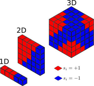
In the Ising model, we consider a collection of spins, $s_{i}$ , each of which can either have the value "up" (+1) or "down" (-1), arranged on a lattice. In one dimension, this takes the form of a "chain" of adjacent spins, $s_{1}$ to $s_{N}$ . In two dimensions we have a grid of cells, each of which contains one spin. In three dimensions, the system is a cuboid, and so on. The arrangements for 1, 2 and 3 dimensions are illustrated in figure 1.

**Figure 1**: Illustration of an Ising lattice in one (N=5), two (N=5x5), and three (N=5x5x5) dimensions. Red cells indicate the "up" spin", and blue cells indicate the "down" spin.

The rules of the model are simple:

When no magnetic field is applied, the only energetic contribution comes from the interaction between spins in adjacent lattice cells
The total interaction energy is defined as $- \frac{1}{2} J \sum_{i}^{N} \sum_{j \in n e i g h b o u r s (i)} s_{i} s_{j}$ , where $J$ is a constant which controls the strength of interaction and the notation $j \in n e i g h b o u r s (i)$ indicates that spin $j$ must lie in a lattice cell adjacent to spin $i$ . The factor of one half is included to make sure that we do not count each spin-spin interaction twice.
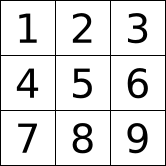
Periodic boundary conditions are applied. In other words, the "final" spin in a particular direction is considered to be adjacent to the "first" spin in that direction. In figure 2, for example, cell 1 has neighbour interactions with cells 2, 3, 4, and 7, while cell 9 interacts with cells 3, 6, 7, and 8.

**Figure 2**: Illustration of a 2D Ising lattice, with numbered cells to indicate the neighbour interactions.

TASK 1a: Show that the lowest possible energy for the Ising model (with $J > 0$ ) is $E = - D N J$ , where $D$ is the number of dimensions and $N$ is the total number of spins. What is the multiplicity of this state? Calculate its entropy.

Phase Transitions

The Ising model is interesting because it is one of the simplest physical models to display a phase transition (so long as we are in two dimensions or more). The temperature of the system controls the balance between the energetic driving force, which wants the system to adopt the lowest energy configuration that you imagined in the previous section, and the entropic driving force, which seeks to maximise the number of configurations available to the system.

TASK 1b: Imagine that the system is in the lowest energy configuration. To move to a different state, one of the spins must spontaneously change direction ("flip"). What is the change in energy if this happens ( $D = 3, N = 1000$ )? How much entropy does the system gain by doing so?

At low temperatures, little thermal energy is available to overcome such energy barriers, and we expect the system to adopt the lowest energy (the energetic driving force will dominate). Under these conditions, we expect a large number of parallel spins, and we can characterise this by considering the total magnetisation of the system: $M = \sum_{i} s_{i}$ . At higher temperatures, however, enough thermal energy will be available that spins can flip relatively freely. Under these conditions, the entropic driving force should dominate. The transition temperature between the two regimes is called the Curie temperature, $T_{C}$ . Below $T_{C}$ , we observe the highly ordered magnetised phase, while above $T_{C}$ a disordered, demagnetised, phase emerges.

TASK 1c: Calculate the magnetisation of the 1D and 2D lattices in figure 1. What magnetisation would you expect to observe for an Ising lattice with $D = 3, N = 1000$ at absolute zero?

We are interested, therefore, in determining the magnetisation $M$ , and energy $E$ , of the system as functions of temperature $T$ . We can write statistical mechanical equations for these quantities:

${⟨ M ⟩}_{T} = \frac{1}{Z} \sum_{α} M (α) \exp {- \frac{E (α)}{k_{B} T}}$

${⟨ E ⟩}_{T} = \frac{1}{Z} \sum_{α} E (α) \exp {- \frac{E (α)}{k_{B} T}}$

where $α$ is used as a shorthand to represent all spins in the system, and $Z$ is the partition function, $Z = \sum_{α} \exp {- \frac{E (α)}{k_{B} T}}$ .

It was discovered relatively quickly after the model was first proposed that the partition function in the one dimensional case can be solved analytically (though doing so is beyond the scope of this experiment):

$Z (T, N) = {[2 \cosh (\frac{J}{k_{B} T})]}^{N}$

Much later, Lars Onsager established that the two dimensional partition function can also be found analytically, though the mathematics is significantly more involved and the resulting expression is correspondingly much more complicated. In dimensions greater than two, no analytical solution is known.

Luckily for us, the problem can instead be tackled by numerical methods, and it is this that will be the focus of the experiment. We will discuss how the equations for $M$ and $E$ can be solved, but first we must set up a Python script to model the lattice.

This is the first section of the Ising model experiment. You can return to the introduction page, or jump ahead to the next section, Calculating the energy and magnetisation.